Innovative approaches of a time-fractional system of Boussinesq equations within a Mohand transform

Meshari Alesemi; Meshari Alesemi

doi:10.3934/math.20241419

AIMS Mathematics

2024, Volume 9, Issue 10: 29269-29295. doi: 10.3934/math.20241419

Previous Article Next Article

Research article Special Issues

Innovative approaches of a time-fractional system of Boussinesq equations within a Mohand transform

Meshari Alesemi ^,

Department of Mathematics, College of Science, University of Bisha, P.O. Box 511, Bisha 61922, Saudi Arabia

Received: 25 August 2024 Revised: 21 September 2024 Accepted: 08 October 2024 Published: 16 October 2024
MSC : 34G20, 35A20, 35A22, 35R11

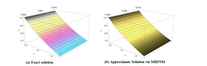
This paper investigated the application of analytical methods, specifically the Mohand transform iterative method (MTIM) and the Mohand residual power series method (MRPSM), to solve the fractional Boussinesq equation. Utilizing the Caputo operator to manage fractional derivatives, these semi-analytical approaches provide accurate solutions to complex fractional differential equations. Through convergence analysis and error estimation, the study validated the efficacy of these methods by comparing numerical solutions to known exact solutions. Graphical and tabular representations illustrated the accuracy of the proposed methods, highlighting their performance for varying fractional orders. The findings demonstrated that both MTIM and MRPSM offer reliable, efficient solutions, making them valuable tools for addressing fractional differential systems in fields such as applied mathematics, engineering, and physics.

Keywords:

Citation: Meshari Alesemi. Innovative approaches of a time-fractional system of Boussinesq equations within a Mohand transform[J]. AIMS Mathematics, 2024, 9(10): 29269-29295. doi: 10.3934/math.20241419

Related Papers:

[1]	Azzh Saad Alshehry, Humaira Yasmin, Ali M. Mahnashi . Analyzing fractional PDE system with the Caputo operator and Mohand transform techniques. AIMS Mathematics, 2024, 9(11): 32157-32181. doi: 10.3934/math.20241544
[2]	Azzh Saad Alshehry, Humaira Yasmin, Ali M. Mahnashi . Exploring fractional Advection-Dispersion equations with computational methods: Caputo operator and Mohand techniques. AIMS Mathematics, 2025, 10(1): 234-269. doi: 10.3934/math.2025012
[3]	Aisha Abdullah Alderremy, Rasool Shah, Nehad Ali Shah, Shaban Aly, Kamsing Nonlaopon . Comparison of two modified analytical approaches for the systems of time fractional partial differential equations. AIMS Mathematics, 2023, 8(3): 7142-7162. doi: 10.3934/math.2023360
[4]	M. Mossa Al-Sawalha, Khalil Hadi Hakami, Mohammad Alqudah, Qasem M. Tawhari, Hussain Gissy . Novel Laplace-integrated least square methods for solving the fractional nonlinear damped Burgers' equation. AIMS Mathematics, 2025, 10(3): 7099-7126. doi: 10.3934/math.2025324
[5]	Nader Al-Rashidi . Innovative approaches to fractional modeling: Aboodh transform for the Keller-Segel equation. AIMS Mathematics, 2024, 9(6): 14949-14981. doi: 10.3934/math.2024724
[6]	Musawa Yahya Almusawa, Hassan Almusawa . Numerical analysis of the fractional nonlinear waves of fifth-order KdV and Kawahara equations under Caputo operator. AIMS Mathematics, 2024, 9(11): 31898-31925. doi: 10.3934/math.20241533
[7]	Emad Salah, Ahmad Qazza, Rania Saadeh, Ahmad El-Ajou . A hybrid analytical technique for solving multi-dimensional time-fractional Navier-Stokes system. AIMS Mathematics, 2023, 8(1): 1713-1736. doi: 10.3934/math.2023088
[8]	Humaira Yasmin, Aljawhara H. Almuqrin . Analytical study of time-fractional heat, diffusion, and Burger's equations using Aboodh residual power series and transform iterative methodologies. AIMS Mathematics, 2024, 9(6): 16721-16752. doi: 10.3934/math.2024811
[9]	Aslı Alkan, Halil Anaç . The novel numerical solutions for time-fractional Fornberg-Whitham equation by using fractional natural transform decomposition method. AIMS Mathematics, 2024, 9(9): 25333-25359. doi: 10.3934/math.20241237
[10]	Thongchai Botmart, Ravi P. Agarwal, Muhammed Naeem, Adnan Khan, Rasool Shah . On the solution of fractional modified Boussinesq and approximate long wave equations with non-singular kernel operators. AIMS Mathematics, 2022, 7(7): 12483-12513. doi: 10.3934/math.2022693

Abstract

1. Introduction

The study of fractional partial differential equations (FPDEs) has garnered significant attention recently due to their ability to model complex physical phenomena more accurately than classical differential equations. Fractional calculus, which generalizes the concept of integer-order differentiation and integration to non-integer orders, has been effectively applied to describe systems with memory, hereditary properties, and non-local interactions ^[1,2,3,4]. These characteristics make fractional equations essential in fluid dynamics, viscoelastic materials, biology, control theory, and signal processing. One such important equation is the fractional Boussinesq equation, which describes wave propagation in shallow water and is instrumental in modeling nonlinear wave phenomena in various media ^[5,6,7,8].

Many problems in the fields of applied sciences, including chemistry and physics, can be effectively solved using fractional calculus (FC), which is often regarded as the best instrument for precisely modeling a range of models. Numerous people have been thinking about the fractional-order control society model lately. Many alternative FC theories with solid mathematical foundations have been considered ^[9,10]. This calculus adequately describes many real-world systems, which is the main reason for its use. Some examples of fractional phenomena are heat conduction, water movement, and infinite lossy transmission lines. Numerous industrial domains use fractional calculus, such as control systems, chemical reactions, electrical circuits, signal processing, chaos theory, and chemical phenomena ^[11,12]. Numerous authors have studied the relationship between the concepts of stability and symmetry in differential equations for a wide range of differential equation systems, such as non-equilibrium statistical mechanics ^[13] and irreversible thermodynamics ^[14]. The relationship between stability and symmetry and the study and control of nonlinear dynamical systems and networks is explored in ^[15]. With differential equations having fractional derivatives, this problem is, therefore, contemporary. The stability of the solutions is acknowledged as one of the most important properties of functional differential equations ^[16,17,18].

In this paper, we focus on solving the fractional-order Boussinesq equation, a model that plays a crucial role in fluid dynamics and nonlinear wave theory. The complexity of fractional derivatives, particularly in systems involving memory effects and hereditary properties, presents challenges that often require sophisticated numerical or analytical techniques to obtain accurate solutions. Traditional methods for solving fractional differential equations (FDEs) are often limited in their applicability or lead to significant computational expense. This underscores the need for more efficient and precise methods to handle such equations ^{[19,20,21,22,23]}. In hydrodynamics, a system of equations known as the Boussinesq equation was created to explain how waves propagate in nonlinear and dissipative media ^[24]. They are frequently used in coastal and ocean engineering to address issues with water percolation in porous subsurface strata. The Boussinesq equation is also the basis for many models that explain subsurface drainage problems and unconfined groundwater flow ^[25,26,27]. Solitons are produced using the cubic Boussinesq equation, first presented in Priestly and Clarkson's writings ^[28]. Kaya ^[29] used the Adomian decomposition approach, which was created in ^[30,31] and extensively used in ^[32], to analyze this problem. Studies of both solitary waves and rational solutions have been conducted for this problem. The suffix on, which indicates that a particle such as a phonon, peakon, coupon, or photon is present, refers to soliton and compaction, respectively, with and without exponential wings.

The residual power series method (RPSM) was founded in 2013 by Omar Abu Arqub ^[33]. It is made up of the residual error function and the Taylor series. An infinite convergence series is the solution to differential equations. Many differential equations have been used as models for novel RPSM algorithms, including Boussinesq differential equations, fuzzy differential equations, the Korteweg-De Vries Burger's equation, and many more ^[34,35,36]. These algorithms aim to achieve accurate and effective approximations. To address this, we employ two powerful semi-analytical techniques: the Mohand transform iterative method (MTIM) and the Mohand residual power series method (MRPSM). These methods, in conjunction with the Caputo fractional derivative, are applied to handle the fractional components of the Boussinesq equation. Both approaches are well-suited to tackle fractional systems' inherent nonlinearity and complexity, providing solutions that converge rapidly and accurately. The MTIM is known for its iterative nature, which refines approximate solutions progressively, while the MRPSM integrates the residual error in each iteration to ensure high accuracy across multiple iterations. These methods are particularly advantageous due to their flexibility, simplicity, and computational efficiency.

This paper's main objective is to demonstrate these methods' effectiveness in solving the fractional Boussinesq equation. Through a detailed analysis of convergence and error estimation, we validate the proposed approaches by comparing the results with known exact solutions. The study also explores the behavior of the solutions under different fractional orders, providing insights into how the fractional terms influence the system's dynamics. The results are presented graphically and in tabular form, highlighting the accuracy and reliability of the solutions obtained.

This work contributes to the growing research on fractional differential equations by offering efficient and accurate problem-solving tools. The findings have significant implications for various scientific and engineering applications, particularly in fields where modeling nonlinearity, memory, and hereditary effects are critical. By presenting a comprehensive analysis of the fractional Boussinesq equation and offering reliable solutions through MTIM and MRPSM, this paper lays the groundwork for further exploration of fractional systems in more complex scenarios.

2. Essential concepts of the Mohand transform

In order to establish the groundwork for this technique, the following are a few fundamental components and principles of the Mohand transform (MT).

Definition 2.1. According to ^[37], the Mohand transform (MT) of the function $\xi(\mu)$ is as follows:

$M[\xi(\mu)] = R(s) = s^2\int_{0}^{\mu}\xi(\mu)e^{-s\mu}d{\mu}, \ \ {k}_{1}\leq s \leq{k}_{2}.$

If $\xi(\mu)$ is the MT of $R(s)$ , then $\xi(\mu)$ is the inverse of R(s).

$M^{-1}[R(s)] = \xi(\mu).$

The inverse Mohand transform (MIT) is the term used to describe $M^{-1}$ in this instance.

Definition 2.2 (^[38]). The Mohand transform equation has the following fractional derivative:

$M[\xi^{p}(\mu)] = s^{p}R(s)-\sum\limits_{k = 0}^{n-1}\frac{\xi^{k}(0)}{s^{k-(p+1)}}, \ 0 < p\leq n.$

Definition 2.3. The subsequent features are associated with MT:

(1) $M[\xi'(\mu)] = sR(s)-s^{2}R(0)$ ,

(2) $M[\xi''(\mu)] = s^{2}R(s)-s^{3}R(0)-s^{2}R'(0)$ ,

(3) $M[\xi^{n}(\mu)] = s^{n}R(s)-s^{n+1}R(0)-s^{n}R'(0)-\cdots-s^{n}R^{n-1}(0)$ .

Lemma 2.4. In regard to the fractional-order derivative of $\xi({{\lambda}}, {{\mu}})$ under the Caputo derivative $D$ with $p > 0$ , the equation $M[R(s)] = \xi({{\lambda}}, {{\mu}})$ describes the MT in this context.

$\begin{equation} M[D_{{{\mu}}}^{r{p}}\xi({{\lambda}}, {{\mu}})] = {s}^{r{p}}R(s)-\sum\limits_{j = 0}^{r-1}{s}^{{p}(r-j)-1}D_{{{\mu}}}^{j{p}}\xi({{\lambda}}, 0), 0 < {p}\leq 1, \end{equation}$

(2.1)

where ${{\lambda}} = ({{\lambda}}_{1}, {{\lambda}}_{2}, \cdots, {{\lambda}}_{p})\in \mathbb{R}^{p}$ , $p\in \mathbb{N}$ , and $D_{{{\mu}}}^{r{p}} = D_{{{\mu}}}^{{p}}.D_{{{\mu}}}^{{p}}.\cdots.D_{{{\mu}}}^{{p}} (r-times).$

Proof. Equation (2.1) can be verified through induction. The following results are obtained when $r = 1$ is inserted into Eq (2.1):

${ M[D_{{{\mu}}}^{{p}}\xi({{\lambda}}, {{\mu}})] = {s}^{2{p}}R(s)-{s}^{2{p}-1}\xi({{\lambda}}, 0)-{s}^{{p}-1}D_{{{\mu}}}^{{p}}\xi({{\lambda}}, 0) }.$

Definition 2.2 indicates that Eq (2.4) is valid for $r = 1$ . When $r = 2$ is substituted into Eq (2.4), the subsequent outcomes are obtained.

$\begin{equation} M[D_{r}^{2{p}}\xi({{\lambda}}, {{\mu}})] = {s}^{2{p}}R(s)-{s}^{2{p}-1}\xi({{\lambda}}, 0)-{s}^{{p}-1}D_{{{\mu}}}^{{p}}\xi({{\lambda}}, 0). \end{equation}$

(2.2)

In Eq (2.2), the left-hand-side (LHS) method is employed to derive the subsequent results.

$\begin{equation} LHS = M[D_{{{\mu}}}^{2{p}}\xi({{\lambda}}, {{\mu}})]. \end{equation}$

(2.3)

We can express Eq (2.3) as follows:

$\begin{equation} LHS = M[D_{{{\mu}}}^{{p}}\xi({{\lambda}}, {{\mu}})]. \end{equation}$

(2.4)

Assume

$\begin{equation} z({{\lambda}}, {{\mu}}) = D_{{{\mu}}}^{{p}}\xi({{\lambda}}, {{\mu}}). \end{equation}$

(2.5)

As a result, Eq (2.4) is transformed into the following form:

$\begin{equation} LHS = M[D_{{{\mu}}}^{{p}}z({{\lambda}}, {{\mu}})]. \end{equation}$

(2.6)

Due to the utilization of the Caputo derivative, Eq (2.6) is modified.

$\begin{equation} LHS = M[J^{1-{p}}z^{'}({{\lambda}}, {{\mu}})]. \end{equation}$

(2.7)

Additional details may be derived from the R-L integral for MT, which is provided by Eq (2.7):

$\begin{equation} LHS = \frac{M[z^{'}({{\lambda}}, {{\mu}})]}{{s}^{1-{p}}}. \end{equation}$

(2.8)

Equation (2.8) is presented in the subsequent form as a result of the differentiability property of the MT:

$\begin{equation} LHS = {s}^{{p}}Z({{\lambda}}, {s})-\frac{z({{\lambda}}, 0)}{{s}^{1-{p}}}. \end{equation}$

(2.9)

The subsequent outcome is obtained by employing Eq (2.5).

$Z({{\lambda}}, {s}) = {s}^{{p}}R(s)-\frac{\xi({{\lambda}}, 0)}{{s}^{1-{p}}}.$

In this case, $M[z({{\mu}}, {{\lambda}})] = Z({{\lambda}}, {s})$ . Thus, Eq (2.9) is modified to the following form:

$\begin{equation} LHS = {s}^{2{p}}R(s)-\frac{\xi({{\lambda}}, 0)}{{s}^{1-2{p}}}-\frac{D_{{{\mu}}}^{{p}}\xi({{\lambda}}, 0)}{{s}^{1-{p}}}. \end{equation}$

(2.10)

Equations (2.4) and (2.10) are both compatible when $r = K$ . Equation (2.4) will be assumed to be valid for $r = K$ . We can now substitute $r = K$ into Eq (2.4).

$\begin{equation} M[D_{{{\mu}}}^{K{p}}\xi({{\lambda}}, {{\mu}})] = {s}^{K{p}}R(s)-\sum\limits_{j = 0}^{K-1}{s}^{{p}(K-j)-1}D_{{{\mu}}}^{j{p}}\xi({{\lambda}}, 0), \ 0 < {p}\leq1. \end{equation}$

(2.11)

The final proof is that Eq (2.4) is valid for $r = K+1$ . Using Eq (2.4), we can state the following:

$\begin{equation} M[D_{{{\mu}}}^{(K+1){p}}\xi({{\lambda}}, {{\mu}})] = {s}^{(K+1){p}}R(s)-\sum\limits_{j = 0}^{K}{s}^{{p}((K+1)-j)-1}D_{{{\mu}}}^{j{p}}\xi({{\lambda}}, 0). \end{equation}$

(2.12)

Taking the left side of Eq (2.12), we can obtain the following.

$\begin{equation} LHS = M[D_{{{\mu}}}^{K{p}}]. \end{equation}$

(2.13)

Let

$D_{{{\mu}}}^{K{p}} = g({{\lambda}}, {{\mu}}).$

From Eq (2.13), the given results are obtained:

$\begin{equation} LHS = M[D_{{{\mu}}}^{{p}}g({{\lambda}}, {{\mu}})]. \end{equation}$

(2.14)

The subsequent result can be obtained by applying the Caputo derivative and the Riemann-Liouville integral to Eq (2.14).

$\begin{equation} LHS = {s}^{{p}}M[D_{{{\mu}}}^{K{p}}\xi({{\lambda}}, {{\mu}})]-\frac{g({{\lambda}}, 0)}{{s}^{1-{p}}}. \end{equation}$

(2.15)

Equation (2.15) can be obtained from Eq (2.11).

$\begin{equation} LHS = {s}^{r{p}}R(s)-\sum\limits_{j = 0}^{r-1}{s}^{{p}(r-j)-1}D_{{{\mu}}}^{j{p}}\xi({{\lambda}}, 0). \end{equation}$

(2.16)

These results were obtained through the application of Eq (2.16).

$LHS = M[D_{{{\mu}}}^{r{p}}\xi({{\lambda}}, 0)].$

Equation (2.4) is valid for $r = K+1$ . For all positive integers, Eq (2.4) is valid when employing the mathematical induction method.

Lemma 2.5. We will consider that the order function $\xi({{\lambda}}, {{\mu}})$ is exponential. The expression $M[\xi({{\lambda}}, {{\mu}})] = R(s)$ is the formula that stands for the MT of $\xi({{\lambda}}, {{\mu}})$ . This is the MFTS form that is used for MT:

$\begin{equation} R(s) = \sum\limits_{r = 0}^{\infty}\frac{\hbar_{r}({{\lambda}})}{s^{r{p}+1}}, s > 0, \end{equation}$

(2.17)

where ${{\lambda}} = (s_{1}, {{\lambda}}_{2}, \cdots, {{\lambda}}_{p})\in\mathbb{R}^{p}, \ p\in \mathbb{N}$ .

Proof. Let us assume that the fractional form of the Taylor series as follows:

$\begin{equation} \xi({{\lambda}}, {{\mu}}) = \hbar_{0}({{\lambda}})+\hbar_{1}({{\lambda}})\frac{{{\mu}}^{{p}}}{\Gamma[{p}+1]}+\hbar_{2}({{\lambda}})\frac{{{\mu}}^{2{p}}}{\Gamma[2{p}+1]}+\cdots. \end{equation}$

(2.18)

Apply MT on Eq (2.18) to obtain:

$M\left[\xi({{\lambda}}, {{\mu}})\right] = M\left[\hbar_{0}({{\lambda}})\right]+M\left[\hbar_{1}({{\lambda}})\frac{{{\mu}}^{{p}}}{\Gamma[{p}+1]}\right]+M\left[\hbar_{1}({{\lambda}}) \frac{{{\mu}}^{2{p}}}{\Gamma[2{p}+1]}\right]+\cdots.$

When the MT's properties are utilized, the following results are obtained:

${M\left[\xi({{\lambda}}, {{\mu}})\right] = \hbar_{0}({{\lambda}})\frac{1}{s}+\hbar_{1}({{\lambda}})\frac{1}{\Gamma[{p}+1]}\frac{1}{s^{{p}+1}}+\hbar_{2}({{\lambda}}) \frac{1}{\Gamma[2{p}+1]}\frac{1}{s^{2{p}+1}}\cdots.}$

Hence, Eq (2.17), a variant of the Taylor series that is particular to MT, is produced. □

Lemma 2.6. With Eq (2.17) the most current version of the Taylor series, we can express the MFPS as $M[\xi(\lambda, \mu)] = R(s)$ .

$\begin{equation} \hbar_{0}({{\lambda}}) = \lim\limits_{s\rightarrow \infty}sR(s) = \xi({{\lambda}}, 0). \end{equation}$

(2.19)

Proof. This is the revised version of the Taylor series:

$\begin{equation} \hbar_{0}({{\lambda}}) = sR(s)-\frac{\hbar_{1}({{\lambda}})}{s^{{p}}}-\frac{\hbar_{2}({{\lambda}})}{s^{2{p}}}-\cdots. \end{equation}$

(2.20)

Take $lim_{x\rightarrow \infty}$ of Eq (2.19) and a quick calculation to yield the required solution, as illustrated in Eq (2.20). □

Theorem 2.7. Assume we have the function $M[\xi({{\lambda}}, {{\mu}})]$ . The following is the MFPS notation for $R(s)$ :

$R(s) = \sum\limits_{r = 0}^{\infty}\frac{\hbar_{r}({{\lambda}})}{{s}^{r{p}+1}}, \ {s} > 0,$

where ${{\lambda}} = ({{\lambda}}_{1}, {{\lambda}}_{2}, \cdots, {{\lambda}}_{p})\in\mathbb{R}^p$ and $p\in\mathbb{N}$ . Then we have

$\hbar_{r}({{\lambda}}) = D_{r}^{r{p}}\xi({{\lambda}}, 0),$

where $D_{{{\mu}}}^{r{p}} = D_{{{\mu}}}^{{p}}.D_{{{\mu}}}^{{p}}.\cdots.D_{{{\mu}}}^{{p}} (r-times)$ .

Proof. Let the Taylor series be in the form:

$\begin{equation} \hbar_{1}({{\lambda}}) = {s}^{{p}+1}R(s)-{s}^{{p}}\hbar_{0}({{\lambda}})-\frac{\hbar_{2}({{\lambda}})}{{s}^{{p}}}-\frac{\hbar_{3}({{\lambda}})}{{s}^{2{p}}}- \cdots. \end{equation}$

(2.21)

We take the $\lim_{{s}\rightarrow \infty}$ of Eq (2.21) to deduce:

$\hbar_{1}({{\lambda}}) = \lim\limits_{{s}\rightarrow \infty}({s}^{{p}+1}R(s)-{s}^{{p}}\hbar_{0}({{\lambda}}))-\lim\limits_{{s}\rightarrow \infty}\frac{\hbar_{2}({{\lambda}})}{{s}^{{p}}} -\lim\limits_{{s}\rightarrow \infty}\frac{\hbar_{3}({{\lambda}})}{{s}^{2{p}}}- \cdots.$

By computing the limit, we have the following equality:

$\begin{equation} \hbar_{1}({{\lambda}}) = \lim\limits_{{s}\rightarrow \infty}({s}^{{p}+1}R(s)-{s}^{{p}}\hbar_{0}({{\lambda}})). \end{equation}$

(2.22)

When Lemma 2.4 is applied to Eq (2.22), the following outcome is obtained:

$\begin{equation} \hbar_{1}({{\lambda}}) = \lim\limits_{{s}\rightarrow \infty}({s}M[D_{{{\mu}}}^{{p}}\xi({{\lambda}}, {{\mu}})]({s})). \end{equation}$

(2.23)

Additional modifications to Eq (2.23) are made by the use of Lemma 2.5:

$\hbar_{1}({{\lambda}}) = D_{{{\mu}}}^{{p}}\xi({{\lambda}}, 0).$

Again, we apply the $\lim_{{s}\rightarrow \infty}$ and the Taylor series to get:

$\hbar_{2}({{\lambda}}) = {s}^{2{p}+1}R(s)-{s}^{2{p}}\hbar_{0}({{\lambda}})-{s}^{{p}}\hbar_{1}({{\lambda}})-\frac{\hbar_{3}({{\lambda}})}{{s}^{{p}}}- \cdots.$

Lemma 2.5 provides this outcome:

$\begin{equation} \hbar_2({{\lambda}}) = \lim\limits_{{s}\rightarrow \infty}{s}({s}^{2{p}}R(s)-{s}^{2{p}-1}\hbar_{0}({{\lambda}})-{s}^{{p}-1}\hbar_{1}({{\lambda}})). \end{equation}$

(2.24)

Using Lemmas 2.4 and 2.6, Eq (2.24) is transformed into:

$\hbar_{2}({{\lambda}}) = D_{{{\mu}}}^{2{p}}\xi({{\lambda}}, 0).$

When we repeat the process, we get

$\hbar_{3}({{\lambda}}) = \lim\limits_{{s}\rightarrow \infty}{s}(M[D_{{{\mu}}}^{2{p}}\xi({{\lambda}}, {p})]({s})).$

To get the final expression, Lemma 2.6 is applied:

$\hbar_{3}({{\lambda}}) = D_{{{\mu}}}^{3{p}}\xi({{\lambda}}, 0).$

In the generalized form, we have:

$\hbar_{r}({{\lambda}}) = D_{{{\mu}}}^{r{p}}\xi({{\lambda}}, 0).$

This theorem describes and illustrates the ideas which influence the convergence of the modified form of the Taylor series. □

Theorem 2.8. Lemma 2.5 provides a formula for MFTS, which may be expressed as follows: $M [\xi({{\mu}}, {{\lambda}})] = R(s)$ . When $|{s}^{a}M[D_{{{\mu}}}^{(K+1){p}}\xi({{\lambda}}, {{\mu}})]|\leq T$ , for all $s > 0$ and $0 < {p} \leq 1$ , the residual $H_K({{\lambda}}, {s})$ of the new MFTS satisfies the following inequality:

$|H_{K}({{\lambda}}, {s})|\leq \frac{T}{{s}^{(K+1){p}+1}}, \ s > 0.$

Proof. Assume $M[D_{{{\mu}}}^{r{p}}\xi({{\lambda}}, {{\mu}})]({s})$ is defined on $s > 0$ for $r = 0, 1, 2, \cdots$ , $K + 1$ and assume $|{s}M[D_{{{\mu}}^{K+1}}\xi({{\lambda}}, \mu)]| \leq T$ . The updated Taylor series can be used to determine this relationship:

$\begin{equation} H_K({{\lambda}}, {s}) = R(s)-\sum\limits_{r = 0}^K\frac{\hbar_r({{\lambda}})}{{s}^{r{p}+1}}. \end{equation}$

(2.25)

Using Theorem 2.7, Eq (2.25) is converted to the following form:

$\begin{equation} H_K({{\lambda}}, {s}) = R(s)-\sum\limits_{r = 0}^{K}\frac{D_{{{\mu}}}^{r{p}}\xi({{\lambda}}, 0)}{{s}^{r{p}+1}}. \end{equation}$

(2.26)

The solution to the problem is to multiply ${s}^{(K+1)a+1}$ on both sides in order to get

$\begin{equation} {s}^{(K+1){p}+1}H_K({{\lambda}}, {s}) = {s}({s}^{(K+1){p}}R(s)-\sum\limits_{r = 0}^{K}{s}^{(K+1-r){p}-1}D_{{{\mu}}}^{r{p}}\xi({{\lambda}}, 0)). \end{equation}$

(2.27)

Lemma 2.4 applied to Eq (2.27) yields the following result:

$\begin{equation} {s}^{(K+1){p}+1}H_K({{\lambda}}, {s}) = {s}M[D_{{{\mu}}}^{(K+1){p}}\xi({{\lambda}}, {{\mu}})]. \end{equation}$

(2.28)

Taking the absolute value, we get

$\begin{equation} |{s}^{(K+1){p}+1}H_K({{\lambda}}, {s})| = |{s}M[D_{{{\mu}}}^{(K+1){p}}\xi({{\lambda}}, {{\mu}})]|. \end{equation}$

(2.29)

The following is the result of applying the condition from Eq (2.29):

$\begin{equation} \frac{-T}{{s}^{(K+1){p}+1}}\leq H_K({{\lambda}}, {s})\leq \frac{T}{{s}^{(K+1){p}+1}}. \end{equation}$

(2.30)

From Eq (2.30), we get

$|H_K({{\lambda}}, {s})|\leq \frac{T}{{s}^{(K+1){p}+1}}.$

Consequently, a novel condition for the series' convergence is deduced. □

3. Combination of the Mohand transform and RPSM method

This section describes how to create the Mohand transform with RPSM to provide an approximate solution to PDEs.

Step 1. Let us assume the PDE:

$\begin{equation} D_{{{\mu}}}^{{p}}\xi({{\lambda}}, {{\mu}})+\vartheta({{\lambda}})N(\xi)-\delta({{\lambda}}, \xi) = 0. \\ \end{equation}$

(3.1)

Step 2. To get the following, MT is applied to both sides of Eq (3.1):

$\begin{equation} M[D_{{{\mu}}}^{{p}}\xi({{\lambda}}, {{\mu}})+\vartheta({{\lambda}})N(\xi)-\delta({{\lambda}}, \xi)] = 0. \\ \end{equation}$

(3.2)

By using Lemma 2.4, we may get:

$\begin{equation} R(s) = \sum\limits_{j = 0}^{q-1}\frac{D_{{{\mu}}}^{j}\xi({{\lambda}}, 0)}{{s}^{j{p}+1}}-\frac{\vartheta({{\lambda}})Y({s})}{{s}^{j{p}}}+\frac{F({{\lambda}}, {s})}{{s}^{j{p}}}, \end{equation}$

(3.3)

where $M[\delta({{\lambda}}, \xi)] = F({{\lambda}}, {s}), M[N(\xi)] = Y({s})$ .

Step 3. After solving Eq (3.3), we have

$R(s) = \sum\limits_{r = 0}^{\infty}\frac{\hbar_r({{\lambda}})}{{s}^{r{p}+1}}, \ {s} > 0.$

Step 4. Observe the fundamental process:

$\hbar_0({{\lambda}}) = \lim\limits_{{s}\rightarrow \infty}{s} R(s) = \xi({{\lambda}}, 0).$

Applying Theorem 2.8 gives us the following result:

$\begin{array}{c} \hbar_1(\lambda) = D_\mu^p \xi(\lambda, 0), \\ \hbar_2(\lambda) = D_\mu^{2 p} \xi(\lambda, 0), \\ \vdots \\ \hbar_w(\lambda) = D_\mu^{w p} \xi(\lambda, 0). \end{array}$

Step 5. The $K^{th}$ truncated series $R(s)$ may be found using the following formula:

$\begin{array}{c} R_{K}(s) = \sum\limits_{r = 0}^{K}\frac{\hbar_r({{\lambda}})}{{s}^{r{p}+1}}, \ {s} > 0, \\ R_{K}(s) = \frac{\hbar_{0}({{\lambda}})}{{s}}+\frac{\hbar_{1}({{\lambda}})}{{s}^{{p}+1}}+\cdots+\frac{\hbar_{w}({{\lambda}})}{{s}^{w{p}+1}}+\sum\limits_{r = w+1}^{K} \frac{\hbar_r({{\lambda}})}{{s}^{r{p}+1}}. \end{array}$

Step 6. Determine the following using the Mohand residual function (MRF) from Eq (3.3), which is not dependent on the $K^{th}$ -truncated Mohand residual function:

$MRes({{\lambda}}, {s}) = R(s)-\sum\limits_{j = 0}^{q-1}\frac{D_{{{\mu}}}^{j}\xi({{\lambda}}, 0)}{{s}^{j{p}+1}}+\frac{\vartheta({{\lambda}})Y({s})}{{s}^{j{p}}}-\frac{F({{\lambda}}, {s})}{{s}^{j{p}}},$

and

$\begin{equation} MRes_{K}({{\lambda}}, {s}) = R_{K}(s)-\sum\limits_{j = 0}^{q-1}\frac{D_{{{\mu}}}^{j}\xi({{\lambda}}, 0)}{{s}^{j{p}+1}}+\frac{\vartheta({{\lambda}})Y({s})}{{s}^{j{p}}}-\frac{F({{\lambda}}, {s})}{{s}^{j{p}}}. \end{equation}$

(3.4)

Step 7. Rather than using its expansion form, Eq (3.4) can be stated in terms of $R_{K}(s)$ :

$\begin{equation} \begin{split} &MRes_{K}({{\lambda}}, {s}) = \Big(\frac{\hbar_{0}({{\lambda}})}{{s}}+\frac{\hbar_{1}({{\lambda}})}{{s}^{{p}+1}}+\cdots+\frac{\hbar_{w}({{\lambda}})}{{s}^{w{p}+1}}+\sum\limits_{r = w+1}^{K} \frac{\hbar_r({{\lambda}})}{{s}^{r{p}+1}}\Big)\\&-\sum\limits_{j = 0}^{q-1}\frac{D_{{{\mu}}}^{j}\xi({{\lambda}}, 0)}{{s}^{j{p}+1}}+\frac{\vartheta({{\lambda}})Y({s})}{{s}^{j{p}}} -\frac{F({{\lambda}}, {s})}{{s}^{j{p}}}. \end{split} \end{equation}$

(3.5)

Step 8. The solution to Eq (3.5) is to multiply ${s}^{K{p}+1}$ on both sides of the above equation:

$\begin{equation} \begin{split} &{s}^{K{p}+1}MRes_{K}({{\lambda}}, {s}) = {s}^{K{p}+1}\Big(\frac{\hbar_{0}({{\lambda}})}{{s}}+\frac{\hbar_{1}({{\lambda}})}{{s}^{{p}+1}}+\cdots+\frac{\hbar_{w}({{\lambda}})}{{s}^{w{p}+1}}+\sum\limits_{r = w+1}^{K} \frac{\hbar_r({{\lambda}})}{{s}^{r{p}+1}}\\&-\sum\limits_{j = 0}^{q-1}\frac{D_{{{\mu}}}^{j}\xi({{\lambda}}, 0)}{{s}^{j{p}+1}}+\frac{\vartheta({{\lambda}})Y({s})}{{s}^{j{p}}} -\frac{F({{\lambda}}, {s})}{{s}^{j{p}}}\Big). \end{split} \end{equation}$

(3.6)

Step 9. The result that follows may be found by using $\lim_{{s}\rightarrow \infty}$ to evaluate Eq (3.6):

$\begin{equation} \begin{split} &\lim\limits_{{s}\rightarrow \infty}{s}^{K{p}+1}MRes_{K}({{\lambda}}, {s}) = \lim\limits_{{s}\rightarrow \infty}{s}^{K{p}+1}\Big(\frac{\hbar_{0}({{\lambda}})}{{s}}+\frac{\hbar_{1}({{\lambda}})}{{s}^{{p}+1}}+\cdots+\frac{\hbar_{w}({{\lambda}})}{{s}^{w{p}+1}}+\sum\limits_{r = w+1}^{K} \frac{\hbar_r({{\lambda}})}{{s}^{r{p}+1}}\\&-\sum\limits_{j = 0}^{q-1}\frac{D_{{{\mu}}}^{j}\xi({{\lambda}}, 0)}{{s}^{j{p}+1}}+\frac{\vartheta({{\lambda}})Y({s})}{{s}^{j{p}}} -\frac{F({{\lambda}}, {s})}{{s}^{j{p}}}\Big). \end{split} \end{equation}$

(3.7)

Step 10. The aforementioned Eq (3.7) can be solved to get the value of $\hbar_K({{\lambda}})$ :

$\lim\limits_{{s}\rightarrow \infty}({s}^{K{p}+1}MRes_{K}({{\lambda}}, {s})) = 0,$

where $K = 1+w, 2+w, \cdots.$

Step 11. In order to get the $K^{th}$ -approximation of Eq (3.3), substitute a $K$ -truncated series of $R(s)$ for the values of $\hbar_K({{\lambda}})$ .

Step 12. Find $R_{K}(s)$ as $\xi_K({{\lambda}}, {{\mu}})$ to get the $K^{th}$ -approximate solution using the MIT.

A new iterative method combined with the Mohand transform

Consider the following PDE shown below:

$\begin{equation} D_{{{\mu}}}^{{p}}{{\xi}}({{\lambda}}, {{\mu}}) = \Upsilon\Big({{\xi}}({{\lambda}}, {{\mu}}), D_{{{\lambda}}}^{\mu}{{\xi}}({{\lambda}}, {{\mu}}) , D_{{{\lambda}}}^{2\mu}{{\xi}}({{\lambda}}, {{\mu}}), D_{{{\lambda}}}^{3\mu}{{\xi}}({{\lambda}}, {{\mu}})\Big), \ 0 < {p}, \mu\leq1, \end{equation}$

(3.8)

with the initial conditions:

$\begin{equation} {{\xi}}({{\lambda}}, 0) = g(\lambda), \end{equation}$

(3.9)

with ${{\xi}}({{\lambda}}, {{\mu}})$ representing the function that we will have to find, while $\Upsilon\Big({{\xi}}({{\lambda}}, {{\mu}}), D_{{{\lambda}}}^{\mu}{{\xi}}({{\lambda}}, {{\mu}}), D_{{{\lambda}}}^{2\mu}{{\xi}}({{\lambda}}, {{\mu}}), D_{{{\lambda}}}^{3\mu}{{\xi}}({{\lambda}}, {{\mu}})\Big)$ is the linear operator or nonlinear operator of ${{\xi}}({{\lambda}}, {{\mu}}), D_{{{\lambda}}}^{\mu}{{\xi}}({{\lambda}}, {{\mu}}), D_{{{\lambda}}}^{2\mu}{{\xi}}({{\lambda}}, {{\mu}})$ , and $D_{{{\lambda}}}^{3\mu}{{\xi}}({{\lambda}}, {{\mu}})$ . Equation (3.8) can be simplified to the following expression by applying the MT to both sides:

$\begin{equation} {M} [{{\xi}}({{\lambda}}, {{\mu}})] = \frac{1}{{s}^{{p}}}\Big(\frac{{\xi}({{\lambda}}, 0)}{{{s}^{1-{p}}}}+{M} \Big[\Upsilon\Big({{\xi}}({{\lambda}}, {{\mu}}), D_{{{\lambda}}}^{\mu}{{\xi}}({{\lambda}}, {{\mu}}), D_{{{\lambda}}}^{2\mu}{{\xi}}({{\lambda}}, {{\mu}}), D_{{{\lambda}}}^{3\mu}{{\xi}}({{\lambda}}, {{\mu}})\Big)\Big]\Big), \end{equation}$

(3.10)

where the result of applying the inverse MT is given below:

$\begin{equation} {{\xi}}({{\lambda}}, {{\mu}}) = {M}^{-1}\Big[\frac{1}{{s}^{{p}}}\Big(\frac{{\xi}({{\lambda}}, 0)}{{{s}^{1-{p}}}}+{M} \Big[\Upsilon\Big({{\xi}}({{\lambda}}, {{\mu}}), D_{{{\lambda}}}^{\mu}{{\xi}}({{\lambda}}, {{\mu}}), D_{{{\lambda}}}^{2\mu}{{\xi}}({{\lambda}}, {{\mu}}), D_{{{\lambda}}}^{3\mu}{{\xi}}({{\lambda}}, {{\mu}})\Big)\Big]\Big)\Big]. \end{equation}$

(3.11)

The infinite series demonstrates the solution that MTIM generates.

$\begin{equation} {{\xi}}({{\lambda}}, {{\mu}}) = \sum\limits_{i = 0}^{\infty}{{\xi}}_{i}. \end{equation}$

(3.12)

The decomposition of the operators $\Upsilon\Big({{\xi}}, D_{{{\lambda}}}^{\mu}{{\xi}}, D_{{{\lambda}}}^{2\mu}{{\xi}}, D_{{{\lambda}}}^{3\mu}{{\xi}}\Big)$ are:

$\begin{equation} \begin{split} &\Upsilon \Big({{\xi}}, D_{{{\lambda}}}^{\mu}{{\xi}}, D_{{{\lambda}}}^{2\mu}{{\xi}}, D_{{{\lambda}}}^{3\mu}{{\xi}}\Big) = \Upsilon \Big({{\xi}}_{0}, D_{{{\lambda}}}^{\mu}{{\xi}}_{0}, D_{{{\lambda}}}^{2\mu}{{\xi}}_{0}, D_{{{\lambda}}}^{3\mu}{{\xi}}_{0}\Big)\\&+ \sum\limits_{i = 0}^{\infty} \left( \Upsilon \Big(\sum\limits_{k = 0}^{i}\Big({{\xi}}_{k}, D_{{{\lambda}}}^{\mu}{{\xi}}_{k}, D_{{{\lambda}}}^{2\mu}{{\xi}}_{k}, D_{{{\lambda}}}^{3\mu}{{\xi}}_{k}\Big)\Big) -\Upsilon \Big(\sum\limits_{k = 1}^{i-1}\Big({{\xi}}_{k}, D_{{{\lambda}}}^{\mu}{{\xi}}_{k}, D_{{{\lambda}}}^{2\mu}{{\xi}}_{k}, D_{{{\lambda}}}^{3\mu}{{\xi}}_{k}\Big)\Big)\right). \end{split} \end{equation}$

(3.13)

By substituting the values of Eqs (3.12) and (3.13) into the original Eq (3.11), we get the following equation:

$\begin{equation} \begin{split} &\sum\limits_{i = 0}^{\infty}{{\xi}}_i({{\lambda}}, {{\mu}}) = {M}^{-1}\Big[ \frac{1}{{s}^{{p}}}\Big( \sum\limits_{k = 0}^{m-1}\frac{{{\xi}}^{(k)}({{\lambda}}, 0)}{{s}^{2-{p}+k}}+{M}[\Upsilon ({{\xi}}_{0}, D_{{{\lambda}}}^{\mu}{{\xi}}_{0}, D_{{{\lambda}}}^{2\mu}{{\xi}}_{0}, D_{{{\lambda}}}^{3\mu}{{\xi}}_{0})]\Big)\Big]\\&+{M}^{-1}\Big[ \frac{1}{{s}^{{p}}}\Big({M}\Big[ \sum\limits_{i = 0}^{\infty}\Big(\Upsilon \sum\limits_{k = 0}^{i}({{\xi}}_{k}, D_{{{\lambda}}}^{\mu}{{\xi}}_{k}, D_{{{\lambda}}}^{2\mu}{{\xi}}_{k}, D_{{{\lambda}}}^{3\mu}{{\xi}}_{k})\Big)\Big]\Big)\Big]\\&-{M}^{-1}\Big[ \frac{1}{{s}^{{p}}}\Big({M}\Big[\Big(\Upsilon \sum\limits_{k = 1}^{i-1}({{\xi}}_{k}, D_{{{\lambda}}}^{\mu}{{\xi}}_{k}, D_{{{\lambda}}}^{2\mu}{{\xi}}_{k}, D_{{{\lambda}}}^{3\mu}{{\xi}}_{k})\Big)\Big]\Big)\Big], \end{split} \end{equation}$

(3.14)

$\begin{equation} \begin{split} &{{\xi}}_0({{\lambda}}, {{\mu}}) = {M}^{-1}\Big[ \frac{1}{{s}^{{p}}}\Big( \sum\limits_{k = 0}^{m-1}\frac{{{\xi}}^{(k)}({{\lambda}}, 0)}{{s}^{2-{p}+k}}\Big)\Big], \\ &{{\xi}}_1({{\lambda}}, {{\mu}}) = {M}^{-1}\Big[ \frac{1}{{s}^{{p}}}\Big( {M}[\Upsilon ({{\xi}}_{0}, D_{{{\lambda}}}^{\mu}{{\xi}}_{0}, D_{{{\lambda}}}^{2\mu}{{\xi}}_{0}, D_{{{\lambda}}}^{3\mu}{{\xi}}_{0})]\Big)\Big], \\ \vdots\\ &{{\xi}}_{m+1}({{\lambda}}, {{\mu}}) = {M}^{-1}\Big[ \frac{1}{{s}^{{p}}}\Big({M}\Big[ \sum\limits_{i = 0}^{\infty}\Big(\Upsilon \sum\limits_{k = 0}^{i}({{\xi}}_{k}, D_{{{\lambda}}}^{\mu}{{\xi}}_{k}, D_{{{\lambda}}}^{2\mu}{{\xi}}_{k}, D_{{{\lambda}}}^{3\mu}{{\xi}}_{k})\Big)\Big]\Big)\Big]\\&-{M}^{-1}\Big[ \frac{1}{{s}^{{p}}}\Big({M}\Big[\Big(\Upsilon \sum\limits_{k = 1}^{i-1}({{\xi}}_{k}, D_{{{\lambda}}}^{\mu}{{\xi}}_{k}, D_{{{\lambda}}}^{2\mu}{{\xi}}_{k}, D_{{{\lambda}}}^{3\mu}{{\xi}}_{k})\Big)\Big]\Big)\Big], \ m = 1, 2, \cdots. \end{split} \end{equation}$

(3.15)

By applying the following formula, the $m$ -terms of Eq (3.8) can be derived analytically:

$\begin{equation} {{\xi}}({{\lambda}}, {{\mu}}) = \sum\limits_{i = 0}^{m-1}{{\xi}}_{i}. \end{equation}$

(3.16)

4. Application of the proposed methods

4.1. Solution of example (4.1) by MRPSM

Consider the cubic Boussinesq equation of fractional order:

$\begin{equation} \begin{split} &D_{\mu}^{p} {\xi}(\lambda, \mu)+2 \frac{\partial ^2{\xi}^3(\lambda, \mu)}{\partial \lambda^2}-\frac{\partial ^2{\xi}(\lambda, \mu)}{\partial \lambda^2}-\frac{\partial ^4{\xi}(\lambda, \mu)}{\partial \lambda^4} = 0, \text { where }\ 1 < p \leq 2, \end{split} \end{equation}$

(4.1)

with the initial conditions:

$\begin{equation} \begin{split} &{\xi}(\lambda, 0) = \frac{1}{\lambda}, \ \ \frac{\partial {\xi}(\lambda, \mu)}{\partial \mu} = -\frac{1}{\lambda^2}.\\ \end{split} \end{equation}$

(4.2)

So, we will take the initial guess as:

$\begin{equation} \begin{split} &{\xi}(\lambda, 0) = \frac{1}{\lambda}-\frac{\mu}{\lambda^2}, \\ \end{split} \end{equation}$

(4.3)

and the exact solution as:

$\begin{equation} \begin{split} &{\xi}(\lambda, \mu) = \frac{1}{\mu+\lambda}.\\ \end{split} \end{equation}$

(4.4)

Equation (4.1) may be solved using MT and Eq (4.3):

$\begin{equation} \begin{split} &{\xi}(\lambda, s)-\frac{\frac{1}{\lambda}-\frac{\mu}{\lambda^2}}{s}+\frac{2}{s^p}\mathcal{M}_{\mu}\Big[\frac{\partial ^2\mathcal{M}_{\mu}^{-1}{\xi}^3(\lambda, s)}{\partial \lambda^2}\Big]-\frac{1}{s^p}\Big[\frac{\partial ^2{\xi}(\lambda, s)}{\partial \lambda^2}\Big]-\frac{1}{s^p}\Big[\frac{\partial ^4{\xi}(\lambda, s)}{\partial \lambda^4}\Big] = 0. \end{split} \end{equation}$

(4.5)

The values of the $k^{th}$ -truncated series are shown below:

$\begin{equation} \begin{split} {\xi}({\lambda}, s) = \frac{\frac{1}{\lambda}-\frac{\mu}{\lambda^2}}{s}+\sum\limits_{r = 1}^{k}\frac{f_{r}({\lambda}, s)}{s^{rp+1}}, \ \ r = 1, 2, 3, 4\cdots.\\ \end{split} \end{equation}$

(4.6)

Using the Mohand residual, one may get

$\begin{equation} \begin{split} &\mathcal{M}_{{\mu}}Res({\lambda}, s) = {\xi}(\lambda, s)-\frac{\frac{1}{\lambda}-\frac{\mu}{\lambda^2}}{s}+\frac{2}{s^p}\mathcal{M}_{\mu}\Big[\frac{\partial ^2\mathcal{M}_{\mu}^{-1}{\xi}^3(\lambda, s)}{\partial \lambda^2}\Big]-\frac{1}{s^p}\Big[\frac{\partial ^2{\xi}(\lambda, s)}{\partial \lambda^2}\Big]-\frac{1}{s^p}\Big[\frac{\partial ^4{\xi}(\lambda, s)}{\partial \lambda^4}\Big] = 0, \end{split} \end{equation}$

(4.7)

and the ${k}^{th}$ -MRFs as

$\begin{equation} \begin{split} &\mathcal{M}_{{\mu}}Res_{k}({\lambda}, s) = {\xi}_{k}(\lambda, s)-\frac{\frac{1}{\lambda}-\frac{\mu}{\lambda^2}}{s}+\frac{2}{s^p}\mathcal{M}_{\mu}\Big[\frac{\partial ^2\mathcal{M}_{\mu}^{-1}{\xi}_{k}^3(\lambda, s)}{\partial \lambda^2}\Big]-\frac{1}{s^p}\Big[\frac{\partial ^2{\xi}_{k}(\lambda, s)}{\partial \lambda^2}\Big]-\frac{1}{s^p}\Big[\frac{\partial ^4{\xi}_{k}(\lambda, s)}{\partial \lambda^4}\Big] = 0. \end{split} \end{equation}$

(4.8)

The following steps may be taken to get the value of $f_{r}({{\lambda}}, s)$ for $r = 1, 2, 3, ...$ . Put the $r^{th}$ -Mohand residual function Eq (4.8) into the $r^{th}$ -truncated series Eq (4.6), and then multiply $s^{r{p}+1}$ by the equation in order to solve the following relation. $\lim_{s\rightarrow \infty}(s^{r{p}+1}){M}_{{\mu}}Res_{\xi, r}({\lambda}, s)) = 0$ for $r = 1, 2, 3, \cdots$ . A few of the terms are given below:

$\begin{equation} \begin{split} & f_{1}({\lambda}, s) = \frac{2 \lambda \left(\lambda ^2+12\right)-6 \left(\lambda ^2+20\right) \mu }{\lambda ^6}, \end{split} \end{equation}$

(4.9)

$\begin{equation} \begin{split} &f_{2}(\lambda, s) = \frac{24 \left(\lambda \left(\lambda ^4+60 \lambda ^2+1680\right)-5 \left(\lambda ^4+84 \lambda ^2+3024\right) \mu \right)}{\lambda ^{10}}, \end{split} \end{equation}$

(4.10)

and so on.

It is necessary to substitute $f_{r}({\lambda}, s)$ in Eq (4.6) in order to obtain

$\begin{equation} \begin{split} &{\xi}(\lambda, s) = \frac{\frac{1}{\lambda}-\frac{\mu}{\lambda^2}}{s}-\frac{\frac{2 \lambda \left(\lambda ^2+12\right)-6 \left(\lambda ^2+20\right) \mu }{\lambda ^6}}{s^{p+1}}-\frac{\frac{24 \left(\lambda \left(\lambda ^4+60 \lambda ^2+1680\right)-5 \left(\lambda ^4+84 \lambda ^2+3024\right) \mu \right)}{\lambda ^{10}}}{s^{2 p+1}}+\cdots. \end{split} \end{equation}$

(4.11)

Using the both-side inverse MT gives us:

$\begin{equation} \begin{split} { {M}^{-1}[{\xi}(\lambda, s)] = {M}^{-1}\bigg[\frac{\frac{1}{\lambda}-\frac{\mu}{\lambda^2}}{s}-\frac{\frac{2 \lambda \left(\lambda ^2+12\right)-6 \left(\lambda ^2+20\right) \mu }{\lambda ^6}}{s^{p+1}}-\frac{\frac{24 \left(\lambda \left(\lambda ^4+60 \lambda ^2+1680\right)-5 \left(\lambda ^4+84 \lambda ^2+3024\right) \mu \right)}{\lambda ^{10}}}{s^{2 p+1}}+\cdots\bigg].} \end{split} \end{equation}$

(4.12)

$\begin{equation} \begin{split} &{\xi}(\lambda, \mu) = \frac{1}{\lambda}-\frac{\mu}{\lambda^2}-\frac{2\mu^{p} \lambda \left(\lambda ^2+12\right)-6 \left(\lambda ^2+20\right) \mu }{\lambda ^6\Gamma(1+p)}\\&-\frac{24 \mu^{2p}\left(\lambda \left(\lambda ^4+60 \lambda ^2+1680\right)-5 \left(\lambda ^4+84 \lambda ^2+3024\right) \mu \right)}{\lambda ^{10}\Gamma(1+2p)}+\cdots. \end{split} \end{equation}$

(4.13)

4.2. Numerical example solution via MTIM

Consider the cubic Boussinesq equation of fractional order:

$\begin{equation} \begin{split} &D_{\mu}^{p} {\xi}(\lambda, \mu) = -2 \frac{\partial ^2{\xi}^3(\lambda, \mu)}{\partial \lambda^2}+\frac{\partial ^2{\xi}(\lambda, \mu)}{\partial \lambda^2}+\frac{\partial ^4{\xi}(\lambda, \mu)}{\partial \lambda^4}, \text { where }\ 1 < p \leq 2, \end{split} \end{equation}$

(4.14)

with the initial conditions:

$\begin{equation} \begin{split} &{\xi}(\lambda, 0) = \frac{1}{\lambda}, \ \ \frac{\partial {\xi}(\lambda, \mu)}{\partial \mu} = -\frac{1}{\lambda^2}. \end{split} \end{equation}$

(4.15)

So, we will take the initial guess as:

$\begin{equation} \begin{split} &{\xi}(\lambda, 0) = \frac{1}{\lambda}-\frac{\mu}{\lambda^2}.\\ \end{split} \end{equation}$

(4.16)

The following is the result that is obtained when the Mohand transform is applied to Eq (4.14):

$\begin{equation} \begin{split} &{M} [D_{\mu}^{p} {\xi}(\lambda, \mu)] = \frac{1}{{s}^{{p}}}\Big(\sum\limits_{k = 0}^{m-1}\frac{{\xi}^{(k)}({\lambda}, 0)}{{s}^{2-{p}+k}} +{M}\Big[-2 \frac{\partial ^2{\xi}^3(\lambda, \mu)}{\partial \lambda^2}+\frac{\partial ^2{\xi}(\lambda, \mu)}{\partial \lambda^2}+\frac{\partial ^4{\xi}(\lambda, \mu)}{\partial \lambda^4}\Big)\Big]\Big). \end{split} \end{equation}$

(4.17)

Based on the application of the MIT to Eq (4.17), the above equation is as follows:

$\begin{equation} \begin{split} &{\xi}(\lambda, \mu) = M^{-1}\Big[\frac{1}{{s}^{{p}}}\Big(\sum\limits_{k = 0}^{m-1}\frac{{\xi}^{(k)}({\lambda}, \eta, 0)}{{s}^{2-{p}+k}} +{M}\Big[-2 \frac{\partial ^2{\xi}^3(\lambda, \mu)}{\partial \lambda^2}+\frac{\partial ^2{\xi}(\lambda, \mu)}{\partial \lambda^2}+\frac{\partial ^4{\xi}(\lambda, \mu)}{\partial \lambda^4}\Big]\Big)\Big]. \end{split} \end{equation}$

(4.18)

Through the process of implementing the Mohand transform in an iterative manner, the following equation can be established:

$\begin{equation*} \begin{split} {\xi}_0(\lambda, \mu) = {M}^{-1}\Big[\frac{1}{{s}^{{p}}}\Big(\sum\limits_{k = 0}^{m-1}\frac{{\xi}^{(k)}({\lambda}, 0)}{{s}^{2-{p}+k}}\Big)\Big] = {M}^{-1}\Big[\frac{{\xi}({\lambda}, 0)}{{s}^2}\Big] = \frac{1}{\lambda}-\frac{\mu}{\lambda^2}. \end{split} \end{equation*}$

Solving Eq (4.14) with the RL integral yields the following results:

$\begin{equation} \begin{split} &{\xi}(\lambda, \mu) = \frac{1}{\lambda}-\frac{\mu}{\lambda^2} +{M}\Big[-2 \frac{\partial ^2{\xi}^3(\lambda, \mu)}{\partial \lambda^2}+\frac{\partial ^2{\xi}(\lambda, \mu)}{\partial \lambda^2}+\frac{\partial ^4{\xi}(\lambda, \mu)}{\partial \lambda^4}\Big]. \end{split} \end{equation}$

(4.19)

For the purpose of obtaining these terms of the solution, we apply the MITM technique.

$\begin{equation} \begin{split} &{\xi}_{0}(\lambda, \mu) = \frac{1}{\lambda}-\frac{\mu}{\lambda^2}, \end{split} \end{equation}$

(4.20)

$\begin{equation} \begin{split} &{\xi}_{1}(\lambda, \mu) = \Big(2 \left(\lambda ^5-3 \lambda ^4 \mu -90 \lambda \mu ^2+42 \mu ^3\right) \mu ^p\Big)/\Big(\lambda ^8 \Gamma (p+1)\Big), \end{split} \end{equation}$

(4.21)

$\begin{equation} \begin{split} &{\xi}_{2}(\lambda, \mu) = \frac{24 \mu ^{2 p}}{\lambda ^{26}} \Big(\Big(\lambda ^{12} \Big(30 \Big(12 \lambda ^2+517\Big) \lambda ^2 \mu ^3+\Big(\lambda ^2+15\Big) \lambda ^7-5 \Big(\lambda ^2+21\Big) \lambda ^6 \mu -2 \Big(308 \lambda ^2+16875\Big) \lambda ^3 \mu ^2\\ &+11484 \lambda \mu ^4-3276 \mu ^5\Big)\Big)/\Big(\Gamma (2 p+1)\Big)+\Big(2 \mu ^p \Big(\lambda ^6 \Big(-28 \lambda ^{11}+252 \lambda ^{10} \mu -540 \Big(49 \lambda ^2-3944\Big) \lambda ^2 \mu ^5\\ &+135 \Big(88-5 \lambda ^2\Big) \lambda ^7 \mu ^2+9 \Big(55 \lambda ^2-6968\Big) \lambda ^6 \mu ^3+12 \Big(6643 \lambda ^2-81000\Big) \lambda ^3 \mu ^4-1426572 \lambda \mu ^6+301644 \mu ^7\Big) \\ &\times \Gamma (p+1) \Gamma (2 p+1)-\Big(6 \Big(\lambda ^5-3 \lambda ^4 \mu -90 \lambda \mu ^2+42 \mu ^3\Big) \Big(5 \lambda ^{10}-40 \lambda ^9 \mu +9720 \lambda ^5 \mu ^3-4620 \Big(\lambda ^2-45\Big) \lambda ^2 \mu ^4\\ &+6 \Big(13 \lambda ^2-380\Big) \lambda ^6 \mu ^2-221760 \lambda \mu ^5+58800 \mu ^6\Big) \mu ^p \Gamma (3 p+1)^2\Big)/\Big(\Gamma (4 p+1)\Big)\Big)\Big)/\Big(\Gamma (p+1)^3 \Gamma (3 p+1)\Big)\Big). \end{split} \end{equation}$

(4.22)

The final solution is:

$\begin{equation} \begin{split} {\xi}(\lambda, \mu) = {\xi}_{0}(\lambda, \mu)+{\xi}_{1}(\lambda, \mu)+{\xi}_{2}(\lambda, \mu)+\cdots, \end{split} \end{equation}$

(4.23)

$\begin{equation} \begin{split} &{\xi}(\lambda, \mu) = \frac{1}{\lambda}-\frac{\mu}{\lambda^2}+\Big(2 \left(\lambda ^5-3 \lambda ^4 \mu -90 \lambda \mu ^2+42 \mu ^3\right) \mu ^p\Big)/\Big(\lambda ^8 \Gamma (p+1)\Big) \\ &+\frac{24 \mu ^{2 p}}{\lambda ^{26}} \Big(\Big(\lambda ^{12} \Big(30 \Big(12 \lambda ^2+517\Big) \lambda ^2 \mu ^3+\Big(\lambda ^2+15\Big) \lambda ^7-5 \Big(\lambda ^2+21\Big) \lambda ^6 \mu -2 \Big(308 \lambda ^2+16875\Big) \lambda ^3 \mu ^2\\ &+11484 \lambda \mu ^4-3276 \mu ^5\Big)\Big)/\Big(\Gamma (2 p+1)\Big)+\Big(2 \mu ^p \Big(\lambda ^6 \Big(-28 \lambda ^{11}+252 \lambda ^{10} \mu -540 \Big(49 \lambda ^2-3944\Big) \lambda ^2 \mu ^5\\ &+135 \Big(88-5 \lambda ^2\Big) \lambda ^7 \mu ^2+9 \Big(55 \lambda ^2-6968\Big) \lambda ^6 \mu ^3+12 \Big(6643 \lambda ^2-81000\Big) \lambda ^3 \mu ^4-1426572 \lambda \mu ^6+301644 \mu ^7\Big) \\ &\times \Gamma (p+1) \Gamma (2 p+1)-\Big(6 \Big(\lambda ^5-3 \lambda ^4 \mu -90 \lambda \mu ^2+42 \mu ^3\Big) \Big(5 \lambda ^{10}-40 \lambda ^9 \mu +9720 \lambda ^5 \mu ^3-4620 \Big(\lambda ^2-45\Big) \lambda ^2 \mu ^4\\ &+6 \Big(13 \lambda ^2-380\Big) \lambda ^6 \mu ^2-221760 \lambda \mu ^5+58800 \mu ^6\Big) \mu ^p \Gamma (3 p+1)^2\Big)/\Big(\Gamma (4 p+1)\Big)\Big)\Big)/\Big(\Gamma (p+1)^3 \Gamma (3 p+1)\Big)\Big) \\ &+\cdots. \end{split} \end{equation}$

(4.24)

The graphical and tabular representations in this study provide a comprehensive view of the accuracy and reliability of the Mohand transform iterative method (MTIM) and the Mohand residual power series method (MRPSM) when applied to the fractional Boussinesq equation. The graphical comparisons between the MRPSM solutions and the exact solutions (see and ) show excellent agreement for fractional order $p = 2$ at $\mu = 0.01$ , validating the effectiveness of the MRPSM. – further illustrate the behavior of the MRPSM solution for various fractional orders $p = 1.4, 1.5$ , and 1.6, depicting how the solution evolves in 2D and 3D spaces. These figures highlight the method's ability to capture the influence of fractional order on the solution, making it a powerful tool for analyzing fractional systems.

Figure 1. MRPSM solution and exact solution comparison of

${\xi(\lambda, \mu)}$ for

$p = 2$ at

$\mu = 0.01$ .

DownLoad: Full-Size Img PowerPoint

Figure 2. MRPSM solution and exact solution comparison of

${\xi(\lambda, \mu)}$ for

$p = 2$ in 2D at

$\mu = 0.01$ .

DownLoad: Full-Size Img PowerPoint

Figure 3. MRPSM solution for various values of fractional order

$p = 1.4, 1.5$ , and 1.6 of

${\xi(\lambda, \mu)}$ at

$\mu = 0.01$ .

DownLoad: Full-Size Img PowerPoint

Figure 4. MRPSM solution in 3D for various values of fractional order

$p = 1.4, 1.5, 1.6$ , and

$2.0$ of

${\xi(\lambda, \mu)}$ at

$\mu = 0.01$ .

DownLoad: Full-Size Img PowerPoint

Figure 5. MRPSM solution in 2D for various values of fractional order

$p = 1.4, 1.5, 1.6$ , and

$2.0$ of

${\xi(\lambda, \mu)}$ at

$\mu = 0.01$ .

DownLoad: Full-Size Img PowerPoint

Similarly, the MTIM solution ( and ) aligns closely with the exact solutions, showcasing its precision for $p = 2$ at $\mu = 0.01$ . explores the MTIM solutions for different fractional orders, again demonstrating the method's adaptability and accuracy across a range of fractional parameters $p = 1.4, 1.5, 1.6$ and $2.0$ at $\mu = 0.01$ .

Figure 6. MTIM solution and exact solution comparison of

${\xi(\lambda, \mu)}$ for

$p = 2$ at

$\mu = 0.01$ .

DownLoad: Full-Size Img PowerPoint

Figure 7. MTIM solution and exact solution comparison of

${\xi(\lambda, \mu)}$ for

$p = 2$ in 2D at

$\mu = 0.01$ .

DownLoad: Full-Size Img PowerPoint

Figure 8. MTIM solution in 2D for various values of fractional order

$p = 1.4, 1.5, 1.6$ , and

$2.0$ of

${\xi(\lambda, \mu)}$ at

$\mu = 0.01$ .

DownLoad: Full-Size Img PowerPoint

The tables provide a quantitative analysis, with and comparing the MRPSM solutions for different fractional orders of $p$ of ${\xi}(\lambda, \mu)$ , supporting the graphical findings. Table 3 highlights the error comparison between the MRPSM and MTIM solutions, confirming that both methods exhibit low error margins, with the MRPSM showing slightly superior performance in certain cases. Overall, the graphical and tabular data reinforce the conclusion that both methods are effective, but MRPSM offers enhanced accuracy in specific fractional scenarios.

Table 1. MRPSM solution comparison for the fractional order

$p$ of

${\xi}(\lambda, \mu)$ .

$\lambda$	$\xi(\lambda, \mu)_{p = 1.4}$	$\xi(\lambda, \mu)_{p = 1.6}$	$\xi(\lambda, \mu)_{p = 2.0}$	$Exact$	$Error_{p = 2.0}$
1	1.041930	1.002870	0.991253	0.990099	1.153850 $\times 10^{-3}$
2	0.498794	0.497936	0.497549	0.497512	3.647340 $\times 10^{-5}$
3	0.332441	0.332298	0.332231	0.332226	4.832371 $\times 10^{-6}$
4	0.249444	0.249399	0.249378	0.249377	1.149512 $\times 10^{-6}$
5	0.199630	0.199610	0.199601	0.199601	3.769759 $\times 10^{-7}$
6	0.166405	0.166394	0.166390	0.166389	1.514955 $\times 10^{-7}$
7	0.142662	0.142656	0.142653	0.142653	7.005697 $\times 10^{-8}$
8	0.124850	0.124846	0.124844	0.124844	3.590433 $\times 10^{-8}$
9	0.110992	0.110989	0.110988	0.110988	1.990453 $\times 10^{-8}$
10	0.099902	0.099901	0.099900	0.099900	1.174007 $\times 10^{-8}$

| Show Table

DownLoad: CSV

Table 2. MRPSM solution comparison for the fractional order

$p$ of

${\xi}(\lambda, \mu)$ .

$\lambda$	$\xi(\lambda, \mu)_{p = 1.4}$	$\xi(\lambda, \mu)_{p = 1.6}$	$\xi(\lambda, \mu)_{p = 2.0}$	$Exact$	$Error_{p = 2.0}$
1	0.992599	0.990862	0.990096	0.990099	2.790916 $\times 10^{-6}$
2	0.497816	0.497609	0.497512	0.497512	1.309079 $\times 10^{-7}$
3	0.332316	0.332255	0.332226	0.332226	2.503602 $\times 10^{-8}$
4	0.249415	0.249389	0.249377	0.249377	7.858480 $\times 10^{-9}$
5	0.199620	0.199607	0.199601	0.199601	3.209642 $\times 10^{-9}$
6	0.166401	0.166393	0.166389	0.166389	1.545901 $\times 10^{-9}$
7	0.142660	0.142656	0.142653	0.142653	8.339015 $\times 10^{-10}$
8	0.124849	0.124845	0.124844	0.124844	4.886407 $\times 10^{-10}$
9	0.110991	0.110989	0.110988	0.110988	3.049892 $\times 10^{-10}$
10	0.099902	0.099900	0.099900	0.099900	2.000754 $\times 10^{-10}$

| Show Table

DownLoad: CSV

Table 3. MRPSM and MTIM solution error comparison of

${\xi}(\lambda, \mu)$ .

$\mu$	$MRPS\;M_{p = 2}$	$MTIM_{p = 2}$	$Exact$	$MRPS\;M\ Error_{p = 2}$	$MTIM\ Error_{p = 2}$
1	0.991253	0.990096	0.990099	1.153850 $\times 10^{-3}$	2.790916 $\times 10^{-6}$
2	0.497549	0.497512	0.497512	3.647340 $\times 10^{-5}$	1.309079 $\times 10^{-7}$
3	0.332231	0.332226	0.332226	4.832371 $\times 10^{-6}$	2.503602 $\times 10^{-8}$
4	0.249378	0.249377	0.249377	1.149512 $\times 10^{-6}$	7.858480 $\times 10^{-9}$
5	0.199601	0.199601	0.199601	3.769759 $\times 10^{-7}$	3.209642 $\times 10^{-9}$
6	0.166390	0.166389	0.166389	1.514955 $\times 10^{-7}$	1.545901 $\times 10^{-9}$
7	0.142653	0.142653	0.142653	7.005697 $\times 10^{-8}$	8.339015 $\times 10^{-10}$
8	0.124844	0.124844	0.124844	3.590433 $\times 10^{-8}$	4.886407 $\times 10^{-10}$
9	0.110988	0.110988	0.110988	1.990453 $\times 10^{-8}$	3.049892 $\times 10^{-10}$
10	0.099900	0.099900	0.099900	1.174007 $\times 10^{-8}$	2.000754 $\times 10^{-10}$

| Show Table

DownLoad: CSV

4.3. Solution of example (4.25) by MRPSM

Consider the system of PDEs of fractional order having a source term of the form:

$\begin{equation} \begin{split} &D_{\mu}^{p} {\xi_{1}}(\lambda, \mu)-\frac{\partial ^2{\xi_{1}}(\lambda, \mu)}{\partial \lambda^2}-{\xi_{2}}(\lambda, \mu)-\frac{1}{4}{\xi_{1}}(\lambda, \mu)+\frac{4}{5} = 0, \\ &D_{\mu}^{p} {\xi_{2}}(\lambda, \mu)-\frac{\partial ^2{\xi_{2}}(\lambda, \mu)}{\partial \lambda^2}-{\xi_{1}}(\lambda, \mu)-\frac{1}{4}{\xi_{2}}(\lambda, \mu)+\frac{4}{5} = 0, \text { where }\ 1 < p \leq 2. \end{split} \end{equation}$

(4.25)

The initial conditions are:

$\begin{equation} \begin{split} &{\xi_{1}}_{0}(\lambda, \mu) = e^\lambda+1, \ \frac{\partial {\xi_{1}}(\lambda, \mu)}{\partial \mu} = \frac{e^\lambda}{2}, \\ &{\xi_{2}}_{0}(\lambda, \mu) = -e^\lambda+1, \ \frac{\partial {\xi_{2}}(\lambda, \mu)}{\partial \mu} = -\frac{e^\lambda}{2}, \end{split} \end{equation}$

(4.26)

we will take the initial guess as:

$\begin{equation} \begin{split} &{\xi_{1}}_{0}(\lambda, \mu) = e^\lambda+1+\frac{\mu e^\lambda}{2}, \\ &{\xi_{2}}_{0}(\lambda, \mu) = -e^\lambda+1-\frac{\mu e^\lambda}{2}, \end{split} \end{equation}$

(4.27)

and the exact solution as:

$\begin{equation} \begin{split} &{\xi_{1}}(\lambda, \mu) = e^{\frac{\mu}{2}+\lambda}+1, \\ &{\xi_{2}}(\lambda, \mu) = -e^{\frac{\mu}{2}+\lambda}+1. \end{split} \end{equation}$

(4.28)

Equation (4.25) may be solved using MT and Eq (4.27):

$\begin{equation} \begin{split} &{\xi_{1}}(\lambda, s)-\frac{e^\lambda+1+\frac{\mu e^\lambda}{2}}{s}-\frac{1}{s^p}\Big[\frac{\partial ^2{\xi_{1}}(\lambda, s)}{\partial \lambda^2}\Big]-\frac{1}{s^p}\Big[{\xi_{2}}(\lambda, s)\Big]-\frac{1}{4s^p}\Big[{\xi_{1}}(\lambda, s)\Big]+\frac{1}{s^{p+1}}\Big[\frac{4}{5}\Big] = 0, \\ &{\xi_{2}}(\lambda, s)-\frac{-e^\lambda+1-\frac{\mu e^\lambda}{2}}{s}-\frac{1}{s^p}\Big[\frac{\partial ^2{\xi_{2}}(\lambda, s)}{\partial \lambda^2}\Big]-\frac{1}{s^p}\Big[{\xi_{1}}(\lambda, s)\Big]-\frac{1}{4s^p}\Big[{\xi_{2}}(\lambda, s)\Big]+\frac{1}{s^{p+1}}\Big[\frac{4}{5}\Big] = 0. \end{split} \end{equation}$

(4.29)

The values of the $k^{th}$ -truncated series are shown below:

$\begin{equation} \begin{split} &{\xi_{1}}({\lambda}, s) = \frac{e^\lambda+1+\frac{\mu e^\lambda}{2}}{s}+\sum\limits_{r = 1}^{k}\frac{f_{r}({\lambda}, s)}{s^{rp+1}}, \ \ r = 1, 2, 3, 4\cdots, \\ &{\xi_{2}}({\lambda}, s) = \frac{-e^\lambda+1-\frac{\mu e^\lambda}{2}}{s}+\sum\limits_{r = 1}^{k}\frac{l_{r}({\lambda}, s)}{s^{rp+1}}, \ \ r = 1, 2, 3, 4\cdots. \end{split} \end{equation}$

(4.30)

Using the Mohand residual, one may get

$\begin{equation} \begin{split} &\mathcal{M}_{{\mu}}Res({\lambda}, s)\\ & = {\xi_{1}}(\lambda, s)-\frac{e^\lambda+1+\frac{\mu e^\lambda}{2}}{s}-\frac{1}{s^p}\Big[\frac{\partial ^2{\xi_{1}}(\lambda, s)}{\partial \lambda^2}\Big]-\frac{1}{s^p}\Big[{\xi_{2}}(\lambda, s)\Big]-\frac{1}{4s^p}\Big[{\xi_{1}}(\lambda, s)\Big] +\frac{1}{s^{p+1}}\Big[\frac{4}{5}\Big] = 0, \\ &\mathcal{M}_{{\mu}}Res({\lambda}, s)\\ & = {\xi_{2}}(\lambda, s)-\frac{-e^\lambda+1-\frac{\mu e^\lambda}{2}}{s}-\frac{1}{s^p}\Big[\frac{\partial ^2{\xi_{2}}(\lambda, s)}{\partial \lambda^2}\Big]-\frac{1}{s^p}\Big[{\xi_{1}}(\lambda, s)\Big]-\frac{1}{4s^p}\Big[{\xi_{2}}(\lambda, s)\Big] +\frac{1}{s^{p+1}}\Big[\frac{4}{5}\Big] = 0, \end{split} \end{equation}$

(4.31)

and the ${k}^{th}$ -MRFs is:

$\begin{equation} \begin{split} &\mathcal{M}_{{\mu}}Res_{k}({\lambda}, s)\\ & = {\xi_{1}}_{k}(\lambda, s)-\frac{e^\lambda+1+\frac{\mu e^\lambda}{2}}{s}-\frac{1}{s^p}\Big[\frac{\partial ^2{\xi_{1}}_{k}(\lambda, s)}{\partial \lambda^2}\Big]-\frac{1}{s^p}\Big[{\xi_{2}}_{k}(\lambda, s)\Big]-\frac{1}{4s^p}\Big[{\xi_{1}}_{k}(\lambda, s)\Big] +\frac{1}{s^{p+1}}\Big[\frac{4}{5}\Big] = 0, \\ &\mathcal{M}_{{\mu}}Res_{k}({\lambda}, s)\\ & = {\xi_{2}}_{k}(\lambda, s)-\frac{-e^\lambda+1-\frac{\mu e^\lambda}{2}}{s}-\frac{1}{s^p}\Big[\frac{\partial ^2{\xi_{2}}_{k}(\lambda, s)}{\partial \lambda^2}\Big]-\frac{1}{s^p}\Big[{\xi_{1}}_{k}(\lambda, s)\Big]-\frac{1}{4s^p}\Big[{\xi_{2}}_{k}(\lambda, s)\Big] +\frac{1}{s^{p+1}}\Big[\frac{4}{5}\Big] = 0. \end{split} \end{equation}$

(4.32)

The following steps may be taken to get the values of $f_{r}({{\lambda}}, s)$ and $l_{r}({{\lambda}}, s)$ for $r = 1, 2, 3, ...$ . Put the $r^{th}$ -Mohand residual function Eq (4.32) into the $r^{th}$ -truncated series Eq (4.30), and then multiply $s^{r{p}+1}$ by the equation in order to solve the following relation: $\lim_{s\rightarrow \infty}(s^{r{p}+1}){M}_{{\mu}}Res_{\xi, r}({\lambda}, s)) = 0$ for $r = 1, 2, 3, \cdots$ . A few of the terms are given below:

$\begin{equation} \begin{split} & f_{1}({\lambda}, s) = \frac{1}{8} e^{\lambda } (\mu +2)+\frac{9}{20}, \\ & l_{1}({\lambda}, s) = \frac{9}{20}-\frac{1}{8} e^{\lambda } (\mu +2), \end{split} \end{equation}$

(4.33)

$\begin{equation} \begin{split} &f_{2}(\lambda, s) = \frac{1}{32} \left((\mu+2) e^\lambda+18\right), \\ &l_{2}(\lambda, s) = \frac{9}{16}-\frac{1}{32} (\mu+2) e^\lambda, \end{split} \end{equation}$

(4.34)

and so on.

It is necessary to substitute $f_{r}({\lambda}, s)$ and $l_{r}({\lambda}, s)$ in Eq (4.30) in order to obtain

$\begin{equation} \begin{split} &{\xi_{1}}(\lambda, s) = \frac{e^\lambda+1+\frac{\mu e^\lambda}{2}}{s}+\frac{\frac{1}{8} e^{\lambda } (\mu +2)+\frac{9}{20}}{s^{p+1}}-\frac{\frac{1}{32} \left((\mu+2) e^\lambda+18\right)}{s^{2 p+1}}+\cdots, \\ &{\xi_{2}}(\lambda, s) = \frac{-e^\lambda+1-\frac{\mu e^\lambda}{2}}{s}+\frac{\frac{9}{20}-\frac{1}{8} e^{\lambda } (\mu +2)}{s^{p+1}}-\frac{\frac{9}{16}-\frac{1}{32} (\mu+2) e^\lambda}{s^{2 p+1}}+\cdots. \end{split} \end{equation}$

(4.35)

Make use of MIT in order to get:

$\begin{equation} \begin{split} &{\xi_{1}}(\lambda, \mu) = 1+\frac{1}{2} e^{\lambda } (\mu +2)+\frac{1}{160} \mu ^p \left(\frac{5 \left(e^{\lambda } (\mu +2)+18\right) \mu ^p}{\Gamma (2 p+1)}+\frac{20 e^{\lambda } (\mu +2)+72}{\Gamma (p+1)}\right)+\cdots, \\ &{\xi_{2}}(\lambda, \mu) = 1-\frac{1}{2} e^{\lambda } (\mu +2)+\frac{1}{160} \mu ^p \left(\frac{72-20 e^{\lambda } (\mu +2)}{\Gamma (p+1)}-\frac{5 \left(e^{\lambda } (\mu +2)-18\right) \mu ^p}{\Gamma (2 p+1)}\right)+\cdots. \end{split} \end{equation}$

(4.36)

4.4. Numerical example solution via MTIM

Consider the system of PDEs of fractional order having a source term of the form:

$\begin{equation} \begin{split} &D_{\mu}^{p} {\xi_{1}}(\lambda, \mu) = \frac{\partial ^2{\xi_{1}}(\lambda, \mu)}{\partial \lambda^2}+{\xi_{2}}(\lambda, \mu)+\frac{1}{4}{\xi_{1}}(\lambda, \mu)-\frac{4}{5}, \\ &D_{\mu}^{p} {\xi_{2}}(\lambda, \mu) = \frac{\partial ^2{\xi_{2}}(\lambda, \mu)}{\partial \lambda^2}+{\xi_{1}}(\lambda, \mu)+\frac{1}{4}{\xi_{2}}(\lambda, \mu)-\frac{4}{5}, \text { where }\ 1 < p \leq 2, \end{split} \end{equation}$

(4.37)

with the initial conditions:

(4.38)

and the initial guess:

$\begin{equation} \begin{split} &{\xi_{1}}_{0}(\lambda, \mu) = e^\lambda+1+\frac{\mu e^\lambda}{2}, \\ &{\xi_{2}}_{0}(\lambda, \mu) = -e^\lambda+1-\frac{\mu e^\lambda}{2}. \end{split} \end{equation}$

(4.39)

The following is the result that is obtained when the Mohand transform is applied to Eq (4.37):

$\begin{equation} \begin{split} &{M} [D_{\mu}^{p} {\xi_{1}}(\lambda, \mu)] = \frac{1}{{s}^{{p}}}\Big(\sum\limits_{k = 0}^{m-1}\frac{{\xi}_{1}^{(k)}({\lambda}, 0)}{{s}^{2-{p}+k}} +{M}\Big[\frac{\partial ^2{\xi_{1}}(\lambda, \mu)}{\partial \lambda^2}+{\xi_{2}}(\lambda, \mu)+\frac{1}{4}{\xi_{1}}(\lambda, \mu)-\frac{4}{5}\Big)\Big]\Big), \\ &{M} [D_{\mu}^{p} {\xi_{2}}(\lambda, \mu)] = \frac{1}{{s}^{{p}}}\Big(\sum\limits_{k = 0}^{m-1}\frac{{\xi}_{2}^{(k)}({\lambda}, 0)}{{s}^{2-{p}+k}} +{M}\Big[\frac{\partial ^2{\xi_{2}}(\lambda, \mu)}{\partial \lambda^2}+{\xi_{1}}(\lambda, \mu)+\frac{1}{4}{\xi_{2}}(\lambda, \mu)-\frac{4}{5}\Big)\Big]\Big). \end{split} \end{equation}$

(4.40)

Based on the application of the MIT to Eq (4.40), the equations that are produced are as follows:

$\begin{equation} \begin{split} &{\xi_{1}}(\lambda, \mu) = M^{-1}\Big[\frac{1}{{s}^{{p}}}\Big(\sum\limits_{k = 0}^{m-1}\frac{{\xi}_{1}^{(k)}({\lambda}, 0)}{{s}^{2-{p}+k}} +{M}\Big[\frac{\partial ^2{\xi_{1}}(\lambda, \mu)}{\partial \lambda^2}+{\xi_{2}}(\lambda, \mu)+\frac{1}{4}{\xi_{1}}(\lambda, \mu)-\frac{4}{5}\Big]\Big)\Big], \\ &{\xi_{2}}(\lambda, \mu) = M^{-1}\Big[\frac{1}{{s}^{{p}}}\Big(\sum\limits_{k = 0}^{m-1}\frac{{\xi}_{2}^{(k)}({\lambda}, 0)}{{s}^{2-{p}+k}} +{M}\Big[\frac{\partial ^2{\xi_{2}}(\lambda, \mu)}{\partial \lambda^2}+{\xi_{1}}(\lambda, \mu)+\frac{1}{4}{\xi_{2}}(\lambda, \mu)-\frac{4}{5}\Big]\Big)\Big]. \end{split} \end{equation}$

(4.41)

Through the process of implementing the Mohand transform in an iterative manner, the following equation can be established:

$\begin{equation*} \begin{split} {\xi_{1}}_0(\lambda, \mu)& = {M}^{-1}\Big[\frac{1}{{s}^{{p}}}\Big(\sum\limits_{k = 0}^{m-1}\frac{{\xi}_{1}^{(k)}({\lambda}, 0)}{{s}^{2-{p}+k}}\Big)\Big] \\& = {M}^{-1}\Big[\frac{{\xi_{1}({\lambda}, 0)}}{{s}^2}\Big] = e^\lambda+1+\frac{\mu e^\lambda}{2}, \\ {\xi_{2}}_0(\lambda, \mu)& = {M}^{-1}\Big[\frac{1}{{s}^{{p}}}\Big(\sum\limits_{k = 0}^{m-1}\frac{{\xi}_{2}^{(k)}({\lambda}, 0)}{{s}^{2-{p}+k}}\Big)\Big]\\ & = {M}^{-1}\Big[\frac{{\xi_{2}}({\lambda}, 0)}{{s}^2}\Big] = -e^\lambda+1-\frac{\mu e^\lambda}{2}. \end{split} \end{equation*}$

Solving Eq (4.37) with the RL integral yields the following results:

$\begin{equation} \begin{split} &{\xi_{1}}(\lambda, \mu) = e^\lambda+1+M\Big[\frac{\partial ^2{\xi_{1}}(\lambda, \mu)}{\partial \lambda^2}+{\xi_{2}}(\lambda, \mu)+\frac{1}{4}{\xi_{1}}(\lambda, \mu)-\frac{4}{5}\Big], \\ &{\xi_{2}}(\lambda, \mu) = -e^\lambda+1+M\Big[\frac{\partial ^2{\xi_{2}}(\lambda, \mu)}{\partial \lambda^2}+{\xi_{1}}(\lambda, \mu)+\frac{1}{4}{\xi_{2}}(\lambda, \mu)-\frac{4}{5}\Big]. \end{split} \end{equation}$

(4.42)

For the purpose of obtaining these terms of the solution, the MITM technique is applied:

$\begin{equation} \begin{split} &{\xi_{1}}_{0}(\lambda, \mu) = e^\lambda+1+\frac{\mu e^\lambda}{2}, \\ &{\xi_{2}}_{0}(\lambda, \mu) = -e^\lambda+1-\frac{\mu e^\lambda}{2}, \end{split} \end{equation}$

(4.43)

$\begin{equation} \begin{split} &{\xi_{1}}_{1}(\lambda, \mu) = \frac{\left(5 e^{\lambda } (\mu +2)+18\right) \mu ^p}{40 \Gamma (p+1)}, \\ &{\xi_{2}}_{1}(\lambda, \mu) = \frac{\left(18-5 e^{\lambda } (\mu +2)\right) \mu ^p}{40 \Gamma (p+1)}, \end{split} \end{equation}$

(4.44)

$\begin{equation} \begin{split} &{\xi_{1}}_{2}(\lambda, \mu) = \frac{\left(e^{\lambda } (\mu +2)+18\right) \mu ^{2 p}}{32 \Gamma (2 p+1)}, \\ &{\xi_{2}}_{2}(\lambda, \mu) = \frac{\left(18-e^{\lambda } (\mu +2)\right) \mu ^{2 p}}{32 \Gamma (2 p+1)}. \end{split} \end{equation}$

(4.45)

The final solution is:

$\begin{equation} \begin{split} &{\xi_1}(\lambda, \mu) = {\xi_1}_{0}(\lambda, \mu)+{\xi_1}_{1}(\lambda, \mu)+{\xi_1}_{2}(\lambda, \mu)+\cdots, \\ &{\xi_2}(\lambda, \mu) = {\xi_2}_{0}(\lambda, \mu)+{\xi_2}_{1}(\lambda, \mu)+{\xi_2}_{2}(\lambda, \mu)+\cdots, \end{split} \end{equation}$

(4.46)

$\begin{equation} \begin{split} &{\xi_1}(\lambda, \mu) = e^\lambda+1+\frac{\mu e^\lambda}{2}+\frac{\left(5 e^{\lambda } (\mu +2)+18\right) \mu ^p}{40 \Gamma (p+1)}+\frac{\left(e^{\lambda } (\mu +2)+18\right) \mu ^{2 p}}{32 \Gamma (2 p+1)}+\cdots, \\ &{\xi_2}(\lambda, \mu) = -e^\lambda+1-\frac{\mu e^\lambda}{2}+\frac{\left(18-5 e^{\lambda } (\mu +2)\right) \mu ^p}{40 \Gamma (p+1)}+\frac{\left(18-e^{\lambda } (\mu +2)\right) \mu ^{2 p}}{32 \Gamma (2 p+1)}+\cdots. \end{split} \end{equation}$

(4.47)

The graphical and tabular results presented in this section offer valuable insights into the accuracy and performance of the applied methods for solving the fractional Boussinesq equation in Example 2. and illustrate the comparison between the approximate solution and the exact solution for ${\xi_1(\lambda, \mu)}$ for $p = 2$ at $\mu = 0.01$ . The close alignment between the two demonstrates the high precision of the approximate method. In particular, the 2D visualization in further emphasizes the method's effectiveness in capturing the correct solution behavior over a range of $\lambda$ . and show a similar comparison for ${\xi_2(\lambda, \mu)}$ for $p = 2$ at $\mu = 0.01$ . The strong agreement between the approximate and exact solutions, as depicted in both 1D and 2D graphs, highlights the robustness of the applied method across multiple variables in the system.

Figure 9. Approximate solution and exact solution comparison of

${\xi_1(\lambda, \mu)}$ for

$p = 2$ at

$\mu = 0.01$ .

DownLoad: Full-Size Img PowerPoint

Figure 10. Approximate solution and exact solution comparison of

${\xi_1(\lambda, \mu)}$ for

$p = 2$ in 2D at

$\mu = 0.01$ .

DownLoad: Full-Size Img PowerPoint

Figure 11. Approximate solution and exact solution comparison of

${\xi_2(\lambda, \mu)}$ for

$p = 2$ at

$\mu = 0.01$ .

DownLoad: Full-Size Img PowerPoint

Figure 12. Approximate solution and exact solution comparison of

${\xi_2(\lambda, \mu)}$ for

$p = 2$ in 2D at

$\mu = 0.01$ .

DownLoad: Full-Size Img PowerPoint

The tabular results, presented in and , offer a more detailed numerical comparison of the MRPSM solutions for different fractional orders of $p$ of ${\xi_{1}}(\lambda, \mu)$ . These tables confirm the effectiveness of the MRPSM approach in yielding accurate solutions across various fractional orders. The consistent accuracy across both ${\xi_{1}}(\lambda, \mu)$ and ${\xi_{2}}(\lambda, \mu)$ for different fractional values underscores the versatility of the method and its potential applicability in solving complex fractional differential equations.

Table 4. MRPSM solution comparison for the fractional order

$p$ of

${\xi_{1}}(\lambda, \mu)$ .

$\lambda$	$\xi(\lambda, \mu)_{p = 1.4}$	$\xi(\lambda, \mu)_{p = 1.6}$	$\xi(\lambda, \mu)_{p = 2.0}$	$Exact$	$Error_{p = 2.0}$
1.0	3.7333191	3.7323733	3.7319298	3.7319072	2.2613496 $\times 10^{-5}$
1.4	5.0773505	5.0761242	5.0755494	5.0755267	2.2669201 $\times 10^{-5}$
1.8	7.0824097	7.0807651	7.0799942	7.0799714	2.2752303 $\times 10^{-5}$
2.2	10.073606	10.071337	10.070274	10.070251	2.2876277 $\times 10^{-5}$
2.6	14.535947	14.532748	14.531248	14.531225	2.3061224 $\times 10^{-5}$
3.0	21.192978	21.188390	21.186239	21.186216	2.3337133 $\times 10^{-5}$
3.4	31.124101	31.117441	31.114319	31.114295	2.3748741 $\times 10^{-5}$
3.8	45.939596	45.929846	45.925274	45.925250	2.4362788 $\times 10^{-5}$
4.2	68.041717	68.027356	68.020622	68.020597	2.5278838 $\times 10^{-5}$
4.6	101.01420	100.99296	100.98300	100.98298	2.6645424 $\times 10^{-5}$
5.0	150.20338	150.17188	150.15711	150.15708	2.8684131 $\times 10^{-5}$

| Show Table

DownLoad: CSV

Table 5. MRPSM solution comparison for the fractional order

$p$ of

${\xi_{2}}(\lambda, \mu)$ .

$\lambda$	$\xi(\lambda, \mu)_{p = 1.4}$	$\xi(\lambda, \mu)_{p = 1.6}$	$\xi(\lambda, \mu)_{p = 2.0}$	$Exact$	$Error_{p = 2.0}$
1.0	-1.7321702	-1.7319760	-1.7318848	-1.7319072	2.2386972 $\times 10^{-5}$
1.4	-3.0762016	-3.0757270	-3.0755044	-3.0755267	2.2331267 $\times 10^{-5}$
1.8	-5.0812607	-5.0803679	-5.0799492	-5.0799714	2.2248165 $\times 10^{-5}$
2.2	-8.0724575	-8.0709407	-8.0702294	-8.0702515	2.2124191 $\times 10^{-5}$
2.6	-12.534798	-12.532351	-12.531203	-12.531225	2.1939243 $\times 10^{-5}$
3.0	-19.191829	-19.187993	-19.186194	-19.186216	2.1663334 $\times 10^{-5}$
3.4	-29.122952	-29.117044	-29.114274	-29.114295	2.1251727 $\times 10^{-5}$
3.8	-43.938447	-43.929448	-43.925229	-43.925250	2.0637680 $\times 10^{-5}$
4.2	-66.040568	-66.026958	-66.020577	-66.020597	1.9721630 $\times 10^{-5}$
4.6	-99.013057	-98.992570	-98.982964	-98.982982	1.8355044 $\times 10^{-5}$
5.0	-148.20223	-148.17148	-148.15706	-148.15708	1.6316337 $\times 10^{-5}$

| Show Table

DownLoad: CSV

5. Conclusions

In this study, we explored the application of the Mohand transform iterative method (MTIM) and the Mohand residual power series method (MRPSM) to solve the fractional-order Boussinesq equation, a fractional system of partial differential equations. By leveraging the Caputo operator for fractional derivatives, we were able to extend traditional methods and provide robust solutions to these complex equations. Our findings confirm that both MTIM and MRPSM are effective and provide reliable techniques for addressing fractional differential equations. The detailed convergence analysis and error estimation demonstrate the accuracy and efficiency of the proposed methods. Additionally, the numerical examples, along with the tabular and graphical presentations, validate the solutions and highlight their practical applicability. The results of this study contribute to the growing body of knowledge in fractional calculus and its applications, offering valuable tools for scientists and engineers dealing with similar complex systems. Future research could further enhance these methods and explore their applications in other domains, potentially leading to new advancements in the field of fractional differential equations.

Acknowledgments

The author is thankful to the Deanship of Graduate Studies and Scientific Research at the University of Bisha for supporting this work through the Fast-Track Research Support Program.

Conflict of interest

The author declares that he has no conflicts of interest.

References

[1]	X. Zhang, Y. Feng, Z. Luo, J. Liu, A spatial sixth-order numerical scheme for solving fractional partial differential equation, Appl. Math. Lett., 159 (2025), 109265. https://doi.org/10.1016/j.aml.2024.109265 doi: 10.1016/j.aml.2024.109265
[2]	O. O. Omotola, A. J. Temiatyo, A. A. Sufiat, S. A. Ezekiel, Application of Mohand transform coupled with homotopy perturbation method to solve Newel-White-Segel equation, Ann. Math. Comput. Sci., 21 (2024), 162–180. https://doi.org/10.56947/amcs.v21.267 doi: 10.56947/amcs.v21.267
[3]	M. Nadeem, S. W. Yao, Solving the fractional heat-like and wave-like equations with variable coefficients utilizing the Laplace homotopy method, Int. J. Numer. Methods Heat Fluid Flow, 31 (2021), 273–292. https://doi.org/10.1108/HFF-02-2020-0111 doi: 10.1108/HFF-02-2020-0111
[4]	A. A. Alderremy, R. Shah, N. Iqbal, S. Aly, K. Nonlaopon, Fractional series solution construction for nonlinear fractional reaction-diffusion Brusselator model utilizing Laplace residual power series, Symmetry, 14 (2022), 1944. https://doi.org/10.3390/sym14091944 doi: 10.3390/sym14091944
[5]	J. Fang, M. Nadeem, M. Habib, S. Karim, H. A. Wahash, A new iterative method for the approximate solution of Klein-Gordon and Sine-Gordon equations, J. Funct. Spaces, 2022 (2022), 5365810. https://doi.org/10.1155/2022/5365810 doi: 10.1155/2022/5365810
[6]	S. Alshammari, M. M. Al-Sawalha, R. Shah, Approximate analytical methods for a fractional-order nonlinear system of Jaulent-Miodek equation with energy-dependent Schrödinger potential, Fractal Fract., 7 (2023), 140. https://doi.org/10.3390/fractalfract7020140 doi: 10.3390/fractalfract7020140
[7]	D. Baleanu, K. Diethelm, E. Scalas, J. J. Trujillo, Fractional calculus: models and numerical methods, Series on Complexity, Nonlinearity and Chaos: Volume 3, World Scientific, 2012. https://doi.org/10.1142/8180
[8]	M. M. Al-Sawalha, A. Khan, O. Y. Ababneh, T. Botmart, Fractional view analysis of Kersten-Krasil'shchik coupled KdV-mKdV systems with non-singular kernel derivatives, AIMS Math., 7 (2022), 18334–18359. https://doi.org/10.3934/math.20221010 doi: 10.3934/math.20221010
[9]	C. Zhu, M. Al-Dossari, S. Rezapour, B. Gunay, On the exact soliton solutions and different wave structures to the (2+1) dimensional Chaffee-Infante equation, Results Phys., 57 (2024), 107431. https://doi.org/10.1016/j.rinp.2024.107431 doi: 10.1016/j.rinp.2024.107431
[10]	S. Guo, S. Wang, Twisted relative Rota-Baxter operators on Leibniz conformal algebras, Commun. Algebra, 52 (2024), 3946–3959. https://doi.org/10.1080/00927872.2024.2337276 doi: 10.1080/00927872.2024.2337276
[11]	X. Xi, J. Li, Z. Wang, H. Tian, R. Yang, The effect of high-order interactions on the functional brain networks of boys with ADHD, Eur. Phys. J. Spec. Top., 233 (2024), 817–829. https://doi.org/10.1140/epjs/s11734-024-01161-y doi: 10.1140/epjs/s11734-024-01161-y
[12]	Z. Wang, M. Chen, X. Xi, H. Tian, R. Yang, Multi-chimera states in a higher order network of FitzHugh-Nagumo oscillators, Eur. Phys. J. Spec. Top., 233 (2024), 779–786. https://doi.org/10.1140/epjs/s11734-024-01143-0 doi: 10.1140/epjs/s11734-024-01143-0
[13]	G. Gallavotti, Breakdown and regeneration of time reversal symmetry in nonequilibrium statistical mechanics, Phys. D, 112 (1998), 250–257. https://doi.org/10.1016/S0167-2789(97)00214-5 doi: 10.1016/S0167-2789(97)00214-5
[14]	B. H. Lavenda, Concepts of stability and symmetry in irreversible thermodynamics. I, Found. Phys., 2 (1972), 161–179. https://doi.org/10.1007/BF00708499 doi: 10.1007/BF00708499
[15]	G. Russo, J. J. E. Slotine, Symmetries, stability, and control in nonlinear systems and networks, Phys. Rev. E, 84 (2011), 041929. https://doi.org/10.1103/PhysRevE.84.041929 doi: 10.1103/PhysRevE.84.041929
[16]	Y. Kai, S. Chen, K. Zhang, Z. Yin, Exact solutions and dynamic properties of a nonlinear fourth-order time-fractional partial differential equation, Waves Random Complex Media, 2022. https://doi.org/10.1080/17455030.2022.2044541
[17]	S. Lin, J. Zhang, C. Qiu, Asymptotic analysis for one-stage stochastic linear complementarity problems and applications, Mathematics, 11 (2023), 482. https://doi.org/10.3390/math11020482 doi: 10.3390/math11020482
[18]	L. Liu, S. Zhang, L. Zhang, G. Pan, J. Yu, Multi-UUV maneuvering counter-game for dynamic target scenario based on fractional-order recurrent neural network, IEEE Trans. Cybernetics, 53 (2023), 4015–4028. https://doi.org/10.1109/TCYB.2022.3225106 doi: 10.1109/TCYB.2022.3225106
[19]	C. Yang, A. M. Wazwaz, Q. Zhou, W. Liu, Transformation of soliton states for a (2+1) dimensional fourth-order nonlinear Schrödinger equation in the Heisenberg ferromagnetic spin chain, Laser Phys., 29 (2019), 035401. https://doi.org/10.1088/1555-6611/aaffc9 doi: 10.1088/1555-6611/aaffc9
[20]	X. Liu, H. Triki, Q. Zhou, M. Mirzazadeh, W. Liu, A. Biswas, et al., Generation and control of multiple solitons under the influence of parameters, Nonlinear Dyn., 95 (2019), 143–150. https://doi.org/10.1007/s11071-018-4556-8 doi: 10.1007/s11071-018-4556-8
[21]	C. Yang, W. Liu, Q. Zhou, D. Mihalache, B. A. Malomed, One-soliton shaping and two-soliton interaction in the fifth-order variable-coefficient nonlinear Schrödinger equation, Nonlinear Dyn., 95 (2019), 369–380. https://doi.org/10.1007/s11071-018-4569-3 doi: 10.1007/s11071-018-4569-3
[22]	E. M. Elsayed, R. Shah, K. Nonlaopon, The analysis of the fractional-order Navier-Stokes equations by a novel approach, J. Funct. Spaces, 2022 (2022), 8979447. https://doi.org/10.1155/2022/8979447 doi: 10.1155/2022/8979447
[23]	A. U. K. Niazi, N. Iqbal, R. Shah, F. Wannalookkhee, K. Nonlaopon, Controllability for fuzzy fractional evolution equations in credibility space, Fractal Fract., 5 (2021), 112. https://doi.org/10.3390/fractalfract5030112 doi: 10.3390/fractalfract5030112
[24]	J. L. Bona, M. Chen, J. C. Saut, Boussinesq equations and other systems for small-amplitude long waves in nonlinear dispersive media: Ⅱ. The nonlinear theory, Nonlinearity, 17 (2004), 925. https://doi.org/10.1088/0951-7715/17/3/010 doi: 10.1088/0951-7715/17/3/010
[25]	B. Mehdinejadiani, H. Jafari, D. Baleanu, Derivation of a fractional Boussinesq equation for modelling unconfined groundwater, Eur. Phys. J. Spec. Top., 222 (2013), 1805–1812. https://doi.org/10.1140/epjst/e2013-01965-1 doi: 10.1140/epjst/e2013-01965-1
[26]	S. E. Serrano, Analytical solutions of the nonlinear groundwater flow equation in unconfined aquifers and the effect of heterogeneity, Water Resour. Res., 31 (1995), 2733–2742. https://doi.org/10.1029/95WR02038 doi: 10.1029/95WR02038
[27]	T. Botmart, R. P. Agarwal, M. Naeem, A. Khan, R. Shah, On the solution of fractional modified Boussinesq and approximate long wave equations with non-singular kernel operators, AIMS Math., 7 (2022), 12483–12513. https://doi.org/10.3934/math.2022693 doi: 10.3934/math.2022693
[28]	P. A. Clarkson, T. J. Priestley, Symmetries of a Generalised Boussinesq equation, IMS Technical Report, 1996.
[29]	D. Kaya, Explicit solutions of generalized nonlinear Boussinesq equations, J. Appl. Math., 1 (2001), 29–37.
[30]	G. Adomian, A review of the decomposition method in applied mathematics, J. Math. Anal. Appl., 135 (1988), 501–544. https://doi.org/10.1016/0022-247X(88)90170-9 doi: 10.1016/0022-247X(88)90170-9
[31]	G. Adomian, Solving frontier problems of physics: the decomposition method, Springer Science and Business Media, Vol. 60, 2013.
[32]	A. M. Wazwaz, Necessary conditions for the appearance of noise terms in decomposition solution series, Appl. Math. Comput., 81 (1997), 265–274. https://doi.org/10.1016/S0096-3003(95)00327-4 doi: 10.1016/S0096-3003(95)00327-4
[33]	O. A. Arqub, Series solution of fuzzy differential equations under strongly generalized differentiability, J. Adv. Res. Appl. Math., 5 (2013), 31–52.
[34]	O. A. Arqub, A. El-Ajou, Z. A. Zhour, S. Momani, Multiple solutions of nonlinear boundary value problems of fractional order: a new analytic iterative technique, Entropy, 16 (2014), 471–493. https://doi.org/10.3390/e16010471 doi: 10.3390/e16010471
[35]	T. Eriqat, A. El-Ajou, M. N. Oqielat, Z. Al-Zhour, S. Momani, A new attractive analytic approach for solutions of linear and nonlinear neutral fractional pantograph equations, Chaos Soliton. Fract., 138 (2020), 109957. https://doi.org/10.1016/j.chaos.2020.109957 doi: 10.1016/j.chaos.2020.109957
[36]	M. Alquran, M. Alsukhour, M. Ali, I. Jaradat, Combination of Laplace transform and residual power series techniques to solve autonomous n-dimensional fractional nonlinear systems, Nonlinear Eng., 10 (2021), 282–292. https://doi.org/10.1515/nleng-2021-0022 doi: 10.1515/nleng-2021-0022
[37]	M. Mohand, A. Mahgoub, The new integral transform "Mohand Transform", Adv. Theor. Appl. Math., 12 (2017), 113–120.
[38]	M. Nadeem, J. H. He, A. Islam, The homotopy perturbation method for fractional differential equations: part 1 Mohand transform, Int. J. Numer. Methods Heat Fluid Flow, 31 (2021), 3490–3504. https://doi.org/10.1108/HFF-11-2020-0703 doi: 10.1108/HFF-11-2020-0703

Reader Comments

Your name:*

Email:*
© 2024 the Author(s), licensee AIMS Press. This is an open access article distributed under the terms of the Creative Commons Attribution License (http://creativecommons.org/licenses/by/4.0)

通讯作者: 陈斌, bchen63@163.com

1.
沈阳化工大学材料科学与工程学院沈阳 110142

AIMS Mathematics

1.8 3.4

Metrics

Article views(627) PDF downloads(45) Cited by(0)

Preview PDF

Download XML

Export Citation

Article outline

Show full outline

Figures and Tables

Figures(12) / Tables(5)

AIMS Mathematics

Innovative approaches of a time-fractional system of Boussinesq equations within a Mohand transform

Related Papers:

Abstract

1. Introduction

2. Essential concepts of the Mohand transform

3. Combination of the Mohand transform and RPSM method

4. Application of the proposed methods

4.1. Solution of example (4.1) by MRPSM

4.2. Numerical example solution via MTIM

4.3. Solution of example (4.25) by MRPSM

4.4. Numerical example solution via MTIM

5. Conclusions

Acknowledgments

Conflict of interest

References

Reader Comments

通讯作者: 陈斌, bchen63@163.com

Metrics

Figures and Tables

Other Articles By Authors

Catalog

AIMS Mathematics

Innovative approaches of a time-fractional system of Boussinesq equations within a Mohand transform

Related Papers:

Abstract

1. Introduction

2. Essential concepts of the Mohand transform

3. Combination of the Mohand transform and RPSM method

4. Application of the proposed methods

4.1. Solution of example (4.1) by MRPSM

4.2. Numerical example solution via MTIM

4.3. Solution of example (4.25) by MRPSM

4.4. Numerical example solution via MTIM

5. Conclusions

Acknowledgments

Conflict of interest

References

Reader Comments

通讯作者: 陈斌, bchen63@163.com

Metrics

Figures and Tables

Other Articles By Authors

Related pages

Tools

Export File

Citation

Format

Content

Catalog