Derivation of some solitary wave solutions for the (3+1)- dimensional pKP-BKP equation via the IME tanh function method

Abeer S. Khalifa; Hamdy M. Ahmed; Niveen M. Badra; Jalil Manafian; Khaled H. Mahmoud; Kottakkaran Sooppy Nisar; Wafaa B. Rabie; Abeer S. Khalifa; Hamdy M. Ahmed; Niveen M. Badra; Jalil Manafian; Khaled H. Mahmoud; Kottakkaran Sooppy Nisar; Wafaa B. Rabie

doi:10.3934/math.20241345

AIMS Mathematics

2024, Volume 9, Issue 10: 27704-27720. doi: 10.3934/math.20241345

Previous Article Next Article

Research article Special Issues

Derivation of some solitary wave solutions for the (3+1)- dimensional pKP-BKP equation via the IME tanh function method

1.
Department of Physics and Engineering Mathematics, Faculty of Engineering, Ain Shams University, Abbassia, Cairo, Egypt
2.
Department of Mathematics, Faculty of Basic Sciences, The German University in Cairo (GUC), Cairo, Egypt
3.
Department of Physics and Engineering Mathematics, Higher Institute of Engineering, El Shorouk Academy, Cairo, Egypt
4.
Department of Applied Mathematics, Faculty of Mathematical Sciences, University of Tabriz, Tabriz, Iran
5.
Natural Sciences Faculty, Lankaran State University, 50, H. Aslanov str., Lankaran, Azerbaijan
6.
Department of Physics, College of Khurma University College, Taif University, Taif 21944, Saudi Arabia
7.
Department of Mathematics, College of Science and Humanities in Alkharj, Prince Sattam Bin Abdulaziz University, Alkharj 11942, Saudi Arabia
8.
Department of Engineering Mathematics and Physics, Higher Institute of Engineering and Technology, Tanta, Egypt

Received: 29 August 2024 Revised: 11 September 2024 Accepted: 14 September 2024 Published: 25 September 2024
MSC : 35B35, 35C07, 35C08, 35C09

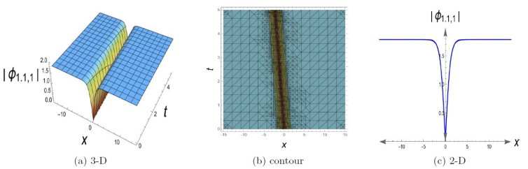
This study is focusing on the integrable (3+1)-dimensional equation that combines the potential Kadomtsev-Petviashvili (pKP) equation with B-type Kadomtsev-Petviashvili (BKP) equation, also known as the pKP-BKP equation. The idea of combining integrable equations has the potential to produce a variety of unexpected outcomes such as resonance of solitons. This article provides a wide range of alternative exact solutions for the pKP-BKP equation in three dimensional form, including dark solitons, singular solitons, singular periodic solutions, Jacobi elliptic function (JEF) solutions, rational solutions and exponential solution. The improved modified extended (IME) tanh function method is employed to investigate these solutions. All of the obtained solutions for the investigated model are presented using the Wolfram Mathematica program. To further help in understanding the solutions' physical characteristics and dynamic structure, the article provides visual representations of some derived solutions using 2D representation in addition to the 3D graphs via symbolic computation. This article aims to use a potent strategy using a powerful scheme to derive different solutions with various structures. Additionally, the results greatly improve and enhance the literature's solutions to a combined pKP-BKP equation and allow deep understanding of the nonlinear dynamic system through different exact solutions.
- potential Kadomtsev-Petviashvili-B-type Kadomtsev-Petviashvili,
- NPDE,
- IME tanh function method,
- solitary wave solutions
Citation: Abeer S. Khalifa, Hamdy M. Ahmed, Niveen M. Badra, Jalil Manafian, Khaled H. Mahmoud, Kottakkaran Sooppy Nisar, Wafaa B. Rabie. Derivation of some solitary wave solutions for the (3+1)- dimensional pKP-BKP equation via the IME tanh function method[J]. AIMS Mathematics, 2024, 9(10): 27704-27720. doi: 10.3934/math.20241345

Related Papers:

Abstract

This study is focusing on the integrable (3+1)-dimensional equation that combines the potential Kadomtsev-Petviashvili (pKP) equation with B-type Kadomtsev-Petviashvili (BKP) equation, also known as the pKP-BKP equation. The idea of combining integrable equations has the potential to produce a variety of unexpected outcomes such as resonance of solitons. This article provides a wide range of alternative exact solutions for the pKP-BKP equation in three dimensional form, including dark solitons, singular solitons, singular periodic solutions, Jacobi elliptic function (JEF) solutions, rational solutions and exponential solution. The improved modified extended (IME) tanh function method is employed to investigate these solutions. All of the obtained solutions for the investigated model are presented using the Wolfram Mathematica program. To further help in understanding the solutions' physical characteristics and dynamic structure, the article provides visual representations of some derived solutions using 2D representation in addition to the 3D graphs via symbolic computation. This article aims to use a potent strategy using a powerful scheme to derive different solutions with various structures. Additionally, the results greatly improve and enhance the literature's solutions to a combined pKP-BKP equation and allow deep understanding of the nonlinear dynamic system through different exact solutions.

References

[1]	H. Li, Y. Zhang, Y. Tai, X. Zhu, X. Qi, L. Zhou, et al., Flexible transparent electromagnetic interference shielding films with silver mesh fabricated using electric-field-driven microscale 3D printing, Opt. Laser Tech., 148 (2022). http://dx.doi.org/10.1016/j.optlastec.2021.107717
[2]	Z. Li, H. Li, X. Zhu, Z. Peng, G. Zhang, J. Yang, et al., Directly printed embedded metal mesh for flexible transparent electrode via liquid substrate electric-field-driven jet, Adv. Sci., 9 (2022), 2105331. http://dx.doi.org/10.1002/advs.202105331 doi: 10.1002/advs.202105331
[3]	X. Zhu, M. Liu, X. Qi, H. Li, Y. Zhang, Z. Li, et al., Templateless, plating-free fabrication of flexible transparent electrodes with embedded silver mesh by electric-field-driven microscale 3D printing and hybrid hot embossing, Adv. Mat., 33 (2021), 2007772. http://dx.doi.org/10.1002/adma.202007772 doi: 10.1002/adma.202007772
[4]	H. Zhang, X. Zhu, Y. Tai, J. Zhou, H. Li, Z. Li, et al., Recent advances in nanofiber-based flexible transparent electrodes, Int. J. Ext. Man., 2023. http://dx.doi.org/10.1088/2631-7990/acdc66
[5]	X. Zhu, Q. Xu, H. Li, M. Liu, Z. Li, K. Yang, et al., Fabrication of high-performance silver mesh for transparent glass heaters via electric-field-driven microscale 3D printing and UV-assisted microtransfer, Adv. Mat., 31 (2019), 1902479. http://dx.doi.org/10.1002/adma.201902479 doi: 10.1002/adma.201902479
[6]	H. Li, Z. Li, N. Li, X. Zhu, Y. Zhang, L. Sun, et al., 3D printed high performance silver mesh for transparent glass heaters through liquid sacrificial substrate electric-field-driven jet, Small, 18 (2022), 2107811. http://dx.doi.org/10.1002/smll.202107811 doi: 10.1002/smll.202107811
[7]	M. Li, T. Wang, F. Chu, Q. Han, Z. Qin, M. J. Zuo, Scaling-Basis chirplet transform, IEEE Trans. Ind. Elec., 68 (2021), 8777–8788. http://dx.doi.org/10.1109/TIE.2020.3013537 doi: 10.1109/TIE.2020.3013537
[8]	H. Jiang, S. M. Li, W. G. Wang, Moderate deviations for parameter estimation in the fractional ornstein-uhlenbeck processes with periodic mean, Acta Math. Sinica, English Ser., 40 (2024), 13081324. http://dx.doi.org/10.1007/s10114-023-2157-z doi: 10.1007/s10114-023-2157-z
[9]	K. K. Ahmed, N. M. Badra, H. M. Ahmed, W. B. Rabie, Unveiling optical solitons and other solutions for fourth-order (2+1)-dimensional nonlinear SchrA dinger equation by modified extended direct algebraic method, J. Opt., 2024, 1–13. http://dx.doi.org/10.1007/s12596-024-01690-8
[10]	A. S. Khalifa, N. M. Badra, H. M. Ahmed, W. B. Rabie, Retrieval of optical solitons in fiber Bragg gratings for high-order coupled system with arbitrary refractive index, Optik, 287 (2023), 171116. http://dx.doi.org/10.1016/j.ijleo.2023.171116 doi: 10.1016/j.ijleo.2023.171116
[11]	W. B. Rabie, K. K. Ahmed, N. M. Badra, H. M. Ahmed, M. Mirzazadeh, M. Eslami, New solitons and other exact wave solutions for coupled system of perturbed highly dispersive CGLE in birefringent fibers with polynomial nonlinearity law, Opt. Quan. Elec., 56 (2024), 875. http://dx.doi.org/10.1007/s11082-024-06644-9 doi: 10.1007/s11082-024-06644-9
[12]	K. K. Ahmed, N. M. Badra, H. M. Ahmed, W. B. Rabie, M. Mirzazadeh, M. Eslami, et al., Investigation of solitons in magneto-optic waveguides with Kudryashovas law nonlinear refractive index for coupled system of generalized nonlinear SchrA dingeras equations using modified extended mapping method, Nonlin. Analy. Model. Cont., 29 (2024), 205–223. http://dx.doi.org/10.15388/namc.2024.29.34070 doi: 10.15388/namc.2024.29.34070
[13]	A. S. Khalifa, H. M. Ahmed, N. M. Badra, W. B. Rabie, Exploring solitons in optical twin-core couplers with Kerr law of nonlinear refractive index using the modified extended direct algebraic method, Opt. Quan. Elec., 56 (2024), 1060. http://dx.doi.org/10.1007/s11082-024-06882-x doi: 10.1007/s11082-024-06882-x
[14]	D. Chen, T. Zhao, L. Han, Z. Feng, Single-stage multi-input buck type high-frequency links inverters with series and simultaneous power supply, IEEE Trans. Power Elec., 37 (2022), 74117421. http://dx.doi.org/10.1109/TPEL.2021.3139646 doi: 10.1109/TPEL.2021.3139646
[15]	C. Chen, D. Han, C. Chang, MPCCT: Multimodal vision-language learning paradigm with context-based compact transformer, Pattern Recogn., 147 (2024), 110084. http://dx.doi.org/10.1016/j.patcog.2023.110084 doi: 10.1016/j.patcog.2023.110084
[16]	H. Wang, D. Han, M. Cui, C. Chen, NAS-YOLOX: A SAR ship detection using neural architecture search and multi-scale attention, Connect. Sci., 35 (2023), 132. http://dx.doi.org/10.1080/09540091.2023.2257399 doi: 10.1080/09540091.2023.2257399
[17]	C. Zhu, X. Li, C. Wang, B. Zhang, B. Li, Deep Learning-Based coseismic deformation estimation from InSAR interferograms, IEEE Trans. Geosci. Remote Sens., 62 (2024), 5203610. http://dx.doi.org/10.1109/TGRS.2024.3357190 doi: 10.1109/TGRS.2024.3357190
[18]	R. Fei, Y. Guo, J. Li, B. Hu, L. Yang, An improved BPNN method based on probability density for indoor location, IEICE Trans. Inf. Syst., 106 (2023), 773785. http://dx.doi.org/10.1587/transinf.2022DLP0073 doi: 10.1587/transinf.2022DLP0073
[19]	K. Zhang, Q. Liu, H. Qian, B. Xiang, Q. Cui, J. Zhou, et al., EATN: An efficient adaptive transfer network for aspect-level sentiment analysis, IEEE Trans. Knowledge Data Eng., 35 (2021), 377389. http://dx.doi.org/10.1109/TKDE.2021.3075238 doi: 10.1109/TKDE.2021.3075238
[20]	D. Chen, T. Zhao, S. Xu, Single-stage multi-input buck type high-frequency links inverters with multiwinding and time-sharing power supply, IEEE Trans. Power Elec., 37 (2022), 12763–12773. http://dx.doi.org/10.1109/TPEL.2022.3176377 doi: 10.1109/TPEL.2022.3176377
[21]	C. Chen, D. Han, X. Shen, CLVIN: Complete language-vision interaction network for visual question answering, Knowl. Based Syst., 275 (2023), 110706. http://dx.doi.org/10.1016/j.knosys.2023.110706 doi: 10.1016/j.knosys.2023.110706
[22]	X. Chen, P. Yang, Y. Peng, M. Wang, F. Hu, J. Xu, Output voltage drop and input current ripple suppression for the pulse load power supply using virtual multiple quasi-notch-flters impedance, IEEE Trans. Power Elec., 38 (2023), 9552–9565. http://dx.doi.org/10.1109/TPEL.2023.3275304 doi: 10.1109/TPEL.2023.3275304
[23]	L. Liao, Z. Guo, Q. Gao, Y. Wang, F. Yu, Q. Zhao, et al., Color image recovery using generalized matrix completion over higher-order finite dimensional algebra, Axioms, 12 (2023), 954. http://dx.doi.org/10.3390/axioms12100954 doi: 10.3390/axioms12100954
[24]	S. Meng, F. Meng, H. Chi, H. Chen, A. Pang, A robust observer based on the nonlinear descriptor systems application to estimate the state of charge of lithium-ion batteries, J. Frankl. Inst., 360 (2023), 11397–11413. http://dx.doi.org/10.1016/j.jfranklin.2023.08.037 doi: 10.1016/j.jfranklin.2023.08.037
[25]	D. L. Chen, J. W. Zhao, S. R. Qin, SVM strategy and analysis of a three-phase quasi-Z-source inverter with high voltage transmission ratio, Sci. China Technol. Sci., 66 (2023), 2996–3010. http://dx.doi.org/10.1007/s11431-022-2394-4 doi: 10.1007/s11431-022-2394-4
[26]	J. Li, H. Tang, X. Li, H. Dou, R. Li, LEF-YOLO: A lightweight method for intelligent detection of four extreme wildfires based on the YOLO framework, Int. J. Wildland Fire, 33 (2023), WF23044. http://dx.doi.org/10.1071/WF23044 doi: 10.1071/WF23044
[27]	T. Wang, S. Zhang, Q. Yang, S. C. Liew, Account service network: A unified decentralized web 3.0 portal with credible anonymity, IEEE Netw., 37 (2023), 101–108. http://dx.doi.org/10.1109/MNET.2023.3321090 doi: 10.1109/MNET.2023.3321090
[28]	J. Dou, J. Liu, Y. Wang, L. Zhi, J. Shen, G. Wang, Surface activity, wetting, and aggregation of a perfuoropolyether quaternary ammonium salt surfactant with a hydroxyethyl group, Molecules, 28 (2023), 7151. http://dx.doi.org/10.3390/molecules28207151 doi: 10.3390/molecules28207151
[29]	J. Hong, L. Gui, J. Cao, Analysis and experimental verification of the tangential force effect on electromagnetic vibration of pm motor, IEEE Trans. Energy Convers., 38 (2023), 1893–1902. http://dx.doi.org/10.1109/TEC.2023.3241082 doi: 10.1109/TEC.2023.3241082
[30]	X. He, Z. Xiong, C. Lei, Z. Shen, A. Ni, Y. Xie, et al., Excellent microwave absorption performance of LaFeO$_3$/Fe$_3$O$_4$/C perovskite composites with optimized structure and impedance matching, Carbon, 213 (2023), 118200. http://dx.doi.org/10.1016/j.carbon.2023.118200 doi: 10.1016/j.carbon.2023.118200
[31]	K. Hosseini, F. Alizadeh, E. HinAsal, M. Ilie, M. S. Osman, Bilinear BA cklund transformation, Lax pair, PainlevA integrability, and different wave structures of a 3D generalized KdV equation, Nonlinear Dyn., 2024, 1–15. http://dx.doi.org/10.1007/s11071-024-09944-7
[32]	K. Hosseini, E. Hincal, K. Sadri, F. Rabiei, M. Ilie, A. Akgül, et al., The positive multi-complexiton solution to a generalized Kadomtseva Petviashvili equation, Par. Diff. Eq. App. Math., 9 (2024), 100647. http://dx.doi.org/10.1016/j.padiff.2024.100647 doi: 10.1016/j.padiff.2024.100647
[33]	Y. Li, S. F. Tian, J. J. Yang, Riemanna Hilbert problem and interactions of solitons in thea component nonlinear SchrA dinger equations, Stud. in App. Math., 148 (2022), 577–605. http://dx.doi.org/10.1111/sapm.12450 doi: 10.1111/sapm.12450
[34]	J. J. Yang, S. F. Tian, Z. Q. Li, Riemanna Hilbert problem for the focusing nonlinear SchrA dinger equation with multiple high-order poles under nonzero boundary conditions, Physica D: Nonlin. Phen., 432 (2022), 133162. http://dx.doi.org/10.1016/j.physd.2022.133162 doi: 10.1016/j.physd.2022.133162
[35]	H. Ma, S. Yue, A. Deng, Lump and interaction solutions for a (2+1)-dimensional combined pKP-BKP equation in fluids, Mod. Phys. Lett. B., 36 (2022), 2250069. http://dx.doi.org/10.1142/S0217984922500695 doi: 10.1142/S0217984922500695
[36]	W. X. Ma, N-soliton solution of a combined pKPa BKP equation, J. Geo. Phys., 165 (2021), 104191. http://dx.doi.org/10.1016/j.geomphys.2021.104191 doi: 10.1016/j.geomphys.2021.104191
[37]	A. M. Wazwaz, New PainlevA integrable (3+1)-dimensional combined pKP-BKP equation: lump and multiple soliton solutions, Chin. Phys. Lett., 40 (2023), 120501. http://dx.doi.org/10.1088/0256-307X/40/12/120501 doi: 10.1088/0256-307X/40/12/120501
[38]	Y. Feng, S. Bilige, Resonant multi-soliton, M-breather, M-lump and hybrid solutions of a combined pKP-BKP equation, J. Geo. Phys., 169 (2021), 104322. http://dx.doi.org/10.1016/j.geomphys.2021.104322 doi: 10.1016/j.geomphys.2021.104322
[39]	Z. Yan, S. Lou, Special types of solitons and breather molecules for a (2+1)-dimensional fifth-order KdV equation, Comm. Nonlin. Sci. Num. Sim., 91 (2020), 105425. http://dx.doi.org/10.1016/j.cnsns.2020.105425 doi: 10.1016/j.cnsns.2020.105425
[40]	M. Kumar, D. V. Tanwar, Lie symmetry reductions and dynamics of solitary wave solutions of breaking soliton equation, Int. J. Geom. Meth. Mod. Phys., 16 (2019), 1950110. http://dx.doi.org/10.1142/S021988781950110X doi: 10.1142/S021988781950110X
[41]	V. I. Kruglov, H. Triki, Interacting solitons, periodic waves and breather for modified kortewega de vries equation, Chin. Phys. Lett., 40 (2023), 090503. http://dx.doi.org/10.1088/0256-307X/40/9/090503 doi: 10.1088/0256-307X/40/9/090503
[42]	X. Liu, Q. Zhou, A. Biswas, A. K. Alzahrani, W. Liu, The similarities and differences of different plane solitons controlled by (3+1) a dimensional coupled variable coefficient system, J. Adv. Res., 24 (2020), 167–173. http://dx.doi.org/10.1016/j.jare.2020.04.003 doi: 10.1016/j.jare.2020.04.003
[43]	R. Hirota, The direct method in soliton theory, Cambridge University Press, 2004. http://dx.doi.org/10.1017/CBO9780511543043
[44]	A. M. Wazwaz, Partial differential equations and solitary waves theory, Springer Berlin: Higher Education Press, 2010. http://dx.doi.org/10.1007/978-3-642-00251-9
[45]	A. M. Wazwaz, Two kinds of multiple wave solutions for the potential YTSF equation and a potential YTSF-type equation, J. Appl. Nonlinear Dyn., 1 (2012), 51–58. https://doi.org/10.5890/JAND.2012.01.001 doi: 10.5890/JAND.2012.01.001
[46]	A. M. Wazwaz, Breather wave solutions for an integrable (3+1)-dimensional combined pKPa BKP equation, Chaos Solit. Fractals, 182 (2024), 114886. https://doi.org/10.1016/j.chaos.2024.114886 doi: 10.1016/j.chaos.2024.114886
[47]	M. B. Almatrafi, Construction of closed form soliton solutions to the space-time fractional symmetric regularized long wave equation using two reliable methods, Fractals, 31 (2023), 2340160. https://doi.org/10.1142/S0218348X23401606 doi: 10.1142/S0218348X23401606
[48]	M. B. Almatrafi, Solitary wave solutions to a fractional model using the improved modified extended tanh-function method, Fractal Fract., 7 (2023), 252. https://doi.org/10.3390/fractalfract7030252 doi: 10.3390/fractalfract7030252
[49]	Y. Cao, Y. Cheng, J. He, Resonant collisions of high-order localized waves in the Maccari system, J. Math. Phys., 64 (2023), 043501. https://doi.org/10.1063/5.0141546 doi: 10.1063/5.0141546
[50]	Y. Cao, J. He, Y. Cheng, The Wronskian, Grammian determinant solutions of a (3+1)-dimensional integrable Kadomtseva Petviashvili equation, Nonlinear Dyn., 111 (2023), 13391–13398. https://doi.org/10.1007/s11071-023-08555-y doi: 10.1007/s11071-023-08555-y
[51]	Y. Cao, J. He, Y. Cheng, Doubly localized twoa dimensional rogue waves generated by resonant collision in Maccari system, Stud. Appl. Math., 152 (2024), 648–672. https://doi.org/10.1111/sapm.12657 doi: 10.1111/sapm.12657
[52]	A. S. Khalifa, W. B. Rabie, N. M. Badra, H. M. Ahmed, M. Mirzazadeh, M. S. Hashemi, et al., Discovering novel optical solitons of two CNLSEs with coherent and incoherent nonlinear coupling in birefringent optical fibers, Opt. Quantum Electron., 56 (2024), 1340. https://doi.org/10.1007/s11082-024-07237-2 doi: 10.1007/s11082-024-07237-2
[53]	K. K. Ahmed, N. M. Badra, H. M. Ahmed, W. B. Rabie, Soliton solutions of generalized Kundu-Eckhaus equation with an extra-dispersion via improved modified extended tanh-function technique, Opt. Quantum Electron., 55 (2023), 299. https://doi.org/10.1007/s11082-023-04599-x doi: 10.1007/s11082-023-04599-x
[54]	K. K. Ahmed, N. M. Badra, H. M. Ahmed, W. B. Rabie, Soliton solutions and other solutions for Kundua Eckhaus equation with quintic nonlinearity and Raman effect using the improved modified extended tanh-function method, Mathematics, 10 (2022), 4203. https://doi.org/10.3390/math10224203 doi: 10.3390/math10224203
[55]	H. Susanto, M. Johansson, Discrete dark solitons with multiple holes, Phys. Rev. E Stat. Nonlin. Soft Matter Phys., 72 (2005), 016605. https://doi.org/10.1103/PhysRevE.72.016605 doi: 10.1103/PhysRevE.72.016605
[56]	A. Maitre, G. Lerario, A. Medeiros, F. Claude, Q. Glorieux, E. Giacobino, et al., Dark-soliton molecules in an exciton-polariton superfluid, Phys. Rev. X., 1 (2020), 041028. https://doi.org/10.1103/PhysRevX.10.041028 doi: 10.1103/PhysRevX.10.041028
[57]	D. V. Douanla, C. G. L. Tiofack, A. Alim, M. Aboubakar, A. Mohamadou, W. Albalawi, et al., Three-dimensional rogue waves and dust-acoustic dark soliton collisions in degenerate ultradense magnetoplasma in the presence of dust pressure anisotropy, Phys. Fluids, 34 (2022), 087105. https://doi.org/10.1063/5.0096990 doi: 10.1063/5.0096990

Reader Comments

Your name:*

Email:*
© 2024 the Author(s), licensee AIMS Press. This is an open access article distributed under the terms of the Creative Commons Attribution License (http://creativecommons.org/licenses/by/4.0)