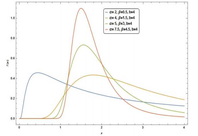
This research introduces a novel right-truncated distribution, termed the right truncated Fréchet-inverted Weibull distribution, and elucidates its mathematical properties including density, cumulative, survival and hazard functions. Various statistical attributes such as moments, quantile, mode and moment-generating functions are explored. These properties indicate the efficiency in modeling pain relief time for patients and the number of recoveries of Leukemia patients. Furthermore, estimation techniques, including maximum likelihood and Bayesian methods, are applied to progressive type-Ⅱ right-censored samples to derive parameter estimation of the proposed distribution. Asymptotic properties are employed to approximate confidence intervals for both reliability and hazard functions. Bayesian estimates are refined using both symmetric and asymmetric loss functions. The suitability of the proposed estimation methodologies is validated through simulation studies. The theoretical framework is applied to two real-world lifetime data sets, thereby substantiating their practical utility in medical areas.
Citation: Nora Nader, Dina A. Ramadan, Hanan Haj Ahmad, M. A. El-Damcese, B. S. El-Desouky. Optimizing analgesic pain relief time analysis through Bayesian and non-Bayesian approaches to new right truncated Fréchet-inverted Weibull distribution[J]. AIMS Mathematics, 2023, 8(12): 31217-31245. doi: 10.3934/math.20231598
This research introduces a novel right-truncated distribution, termed the right truncated Fréchet-inverted Weibull distribution, and elucidates its mathematical properties including density, cumulative, survival and hazard functions. Various statistical attributes such as moments, quantile, mode and moment-generating functions are explored. These properties indicate the efficiency in modeling pain relief time for patients and the number of recoveries of Leukemia patients. Furthermore, estimation techniques, including maximum likelihood and Bayesian methods, are applied to progressive type-Ⅱ right-censored samples to derive parameter estimation of the proposed distribution. Asymptotic properties are employed to approximate confidence intervals for both reliability and hazard functions. Bayesian estimates are refined using both symmetric and asymmetric loss functions. The suitability of the proposed estimation methodologies is validated through simulation studies. The theoretical framework is applied to two real-world lifetime data sets, thereby substantiating their practical utility in medical areas.

| [1] | M. Fréchet, Sur la loi de probabilité de l'écart maximum, Ann. Soc. Math. Polon., 6 (1927), 93–116. |
| [2] |
N. Balakrishnan, Progressive censoring methodology: An appraisal, Test, 16 (2007), 211–259. https://doi.org/10.1007/s11749-007-0061-y doi: 10.1007/s11749-007-0061-y

|
| [3] |
G. M. Cordeiro, A. J. Lemonte, On the Marshall-Olkin extended Weibull distribution, Stat. Pap., 54 (2013), 333–353. https://doi.org/10.1007/s00362-012-0431-8 doi: 10.1007/s00362-012-0431-8
|
| [4] |
Z. Behdani, G. R. M. Borzadaran, B. Gildeh, Some properties of double truncated distributions and their application in view of income inequality, Comput. Stat., 35 (2020), 359–378. https://doi.org/10.1007/s00180-019-00890-2 doi: 10.1007/s00180-019-00890-2
|
| [5] |
L. Zaninetti, A right and left truncated gamma distribution with application to the stars, Adv. Stud. Theor. Phys., 23 (2013), 1139–1147. https://doi.org/10.12988/astp.2013.310125 doi: 10.12988/astp.2013.310125
|
| [6] | M. A. El-Din, A. M. Teamah, A. M. Salem, A. M. T. A. El-Bar, Random sum of mid truncated Lindley distribution, J. Adv. Res. Stat. Probab., 2 (2010), 27–36. |
| [7] |
R. Aggarwala, N. Balakrishnan, Recurrence relations for single and product moments of progressive Type-Ⅱ right censored order statistics from exponential and truncated exponential distributions, Ann. Inst. Stat. Math., 48 (2010), 757–771. https://doi.org/10.1007/BF00052331 doi: 10.1007/BF00052331
|
| [8] | N. Balakrishnan, E. Cramer, The art of progressive censoring, Birkhäuser: NewYork, NY, USA, 2014. |
| [9] | W. Q. Meeker, L. A. Escobar, F. G. Pascual, Statistical methods for reliability data, John Wiley & Sons: Hoboken, NJ, USA, 2022. |
| [10] | N. R. Mann, R. E. Schafer, N. D. Singpurwalla, Methods for statistical analysis of reliability and life data, Research Supported by the U. S. Air Force and Rockwell International Corp, New York, John Wiley and Sons, Inc.: Hoboken, NJ, USA, 1974,573. |
| [11] | J. F. Lawless, Statistical models and methods for lifetime data, Wiley: New York, NY, USA, 1982. |
| [12] |
M. M. Buzaridah, D. A. Ramadan, B. S. El-Desouky, Flexible reduced logarithmic-inverse lomax distribution with application for bladder cancer, Open J. Modell. Simul., 9 (2021), 351–369. https://doi.org/10.4236/ojmsi.2021.94023 doi: 10.4236/ojmsi.2021.94023
|
| [13] |
G. C. Montanari, M. Mazzanti, M. Cacciari, J. C. Fothergill, Optimum estimators for the Weibull distribution from censored test data. Progressively censored tests [breakdown statistics], IEEE Trans. Dielectr. Electr. Insul., 5 (2021), 157–164. https://doi.org/10.1109/94.671923 doi: 10.1109/94.671923
|
| [14] |
I. Bairamov, S. Eryılmaz, Spacings, exceedances and concomitants in progressive type Ⅱ censoring scheme, J. Stat. Plan. Infer., 136 (2006), 527–536. https://doi.org/10.1016/j.jspi.2004.09.002 doi: 10.1016/j.jspi.2004.09.002
|
| [15] |
M. A. W. Mahmoud, D. A. Ramadan, M. M. M. Mansour, Estimation of lifetime parameters of the modified extended exponential distribution with application to a mechanical model, Commun. Stat. Simul. Comput., 1 (2022), 7005–7018. https://doi.org/10.1080/03610918.2020.1821887 doi: 10.1080/03610918.2020.1821887
|
| [16] | D. A. Ramadan, M. Walaa, Estimation of parameters of Alpha power inverse Weibull distribution under progressive type-Ⅱ censoring, J. Stat. Appl. Probab. Lett., 6 (2019), 81–87. |
| [17] |
H. H. Ahmad, E. M. Almetwally, D. A. Ramadan, A comparative inference on reliability estimation for a multi-component stress-strength model under power Lomax distribution with applications, AIMS Math., 7 (2022), 18050–18079. https://doi.org/10.3934/math.2022994 doi: 10.3934/math.2022994
|
| [18] |
H. H. Ahmad, K. Elnagar, D. Ramadan, Investigating the lifetime performance index under ishita distribution based on progressive type Ⅱ censored data with applications, Symmetry, 15 (2023), 1779. https://doi.org/10.3390/sym15091779 doi: 10.3390/sym15091779
|
| [19] |
M. Shrahili, A. Naif, K. Devendra, A. Salem, Inference for the two-parameter reduced Kies distribution under progressive type-Ⅱ censoring, Mathematics, 8 (2020), 1997. https://doi.org/10.3390/math8111997 doi: 10.3390/math8111997
|
| [20] |
C. Luo, L. Shen, A. Xu, Modelling and estimation of system reliability under dynamic operating environments and lifetime ordering constraints, Reliab. Eng. Syst. Saf., 218 (2022), 108–136. https://doi.org/10.1016/j.ress.2021.108136 doi: 10.1016/j.ress.2021.108136
|
| [21] |
M. M. Buzaridah, D. A. Ramadan, B. S. El-Desouky, Estimation of some lifetime parameters of flexible reduced logarithmic-inverse lomax distribution under progressive type-Ⅱ censored, Data. J. Math., 2022 (2022). https://doi.org/10.1155/2022/1690458 doi: 10.1155/2022/1690458
|
| [22] |
J. J. A. Moors, A quantile alternative for kurtosis, J. Roy. Stat. Soc. D-Sta., 37 (1988), 25–32. https://doi.org/10.2307/2348376 doi: 10.2307/2348376
|
| [23] |
R. Aggarwala, N. Balakrishnan, Some properties of progressive censored order statistics from arbitrary and uniform distributions with applications to inference and simulation, J. Stat. Plan. Infer., 70 (1998), 35–49. https://doi.org/10.1016/S0378-3758(97)00173-0 doi: 10.1016/S0378-3758(97)00173-0
|
| [24] | W. Greene, Discrete choice modeling, In: Palgrave Handbook of Econometrics, Palgrave Macmillan: London, UK, 2009,473–556. |
| [25] |
A. Zellner, Bayesian estimation and prediction using asymmetric loss functions, J. Am. Stat. Assoc., 81 (1998), 446–451. https://doi.org/10.1080/01621459.1986.10478289 doi: 10.1080/01621459.1986.10478289
|
| [26] | P. F. Heil, A. J. Gross, V. Clark, Survival distributions: Reliability applications in the biomedical sciences, John Wiley & Sons: Hoboken, NJ, USA, 18 (1975), 501. https://doi.org/10.2307/1268667 |
| [27] |
A. M. Abouammoh, S. A. Abdulghani, I. S. Qamber, On partial orderings and testing of new better than renewal used classes, Reliab. Eng. Syst. Safe., 43 (1994), 37–41. https://doi.org/10.1016/0951-8320(94)90094-9 doi: 10.1016/0951-8320(94)90094-9
|


Figures(8) / Tables(15)

Nora Nader, Dina A. Ramadan, Hanan Haj Ahmad, M. A. El-Damcese, B. S. El-Desouky. Optimizing analgesic pain relief time analysis through Bayesian and non-Bayesian approaches to new right truncated Fréchet-inverted Weibull distribution[J]. AIMS Mathematics, 2023, 8(12): 31217-31245. doi: 10.3934/math.20231598


 DownLoad: