Analysis of progressive Type-Ⅱ censoring schemes for generalized power unit half-logistic geometric distribution

Ahmed R. El-Saeed; Ahmed T. Ramadan; Najwan Alsadat; Hanan Alohali; Ahlam H. Tolba; Ahmed R. El-Saeed; Ahmed T. Ramadan; Najwan Alsadat; Hanan Alohali; Ahlam H. Tolba

doi:10.3934/math.20231577

AIMS Mathematics

2023, Volume 8, Issue 12: 30846-30874. doi: 10.3934/math.20231577

Previous Article Next Article

Research article Special Issues

Analysis of progressive Type-Ⅱ censoring schemes for generalized power unit half-logistic geometric distribution

1.
Department of Basic Sciences, Obour High Institute for Management & Informatics, Egypt
2.
Department of Basic Sciences, High Raya Institute, Damietta 34511, Egypt
3.
Department of Quantitative Analysis, College of Business Administration, King Saud University, P.O. Box 71115, Riyadh 11587, Saudi Arabia
4.
Department of Mathematics, College of Science, King Saud University, P.O. Box 2455, Riyadh 11451, Saudi Arabia
5.
Department of Mathematics, Faculty of Science, Mansoura University, Mansoura 35516, Egypt

Received: 30 August 2023 Revised: 30 October 2023 Accepted: 05 November 2023 Published: 15 November 2023
MSC : 62F15, 62G20, 65C60

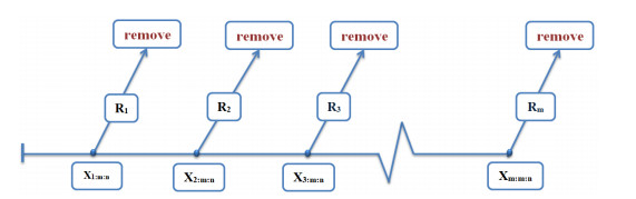
This study addresses the difficulties associated with parameter estimation in the generalized power unit half-logistic geometric distribution by employing a progressive Type-Ⅱ censoring technique. The study uses a variety of methods, including maximum likelihood, maximum product of spacing, and Bayesian estimation. The work investigates Bayesian estimators taking into account a gamma prior and a symmetric loss function while working with observed data produced by likelihood and spacing functions. A full simulation experiment is carried out with varying sample sizes and censoring mechanisms in order to thoroughly evaluate the various estimation approaches. The highest posterior density approach is employed in the study to compute credible intervals for the parameters. Additionally, based on three optimal criteria, the study chooses the best progressive censoring scheme from a variety of rival methods. The study examines two real datasets in order to confirm the applicability of the generalized power unit half-logistic geometric distribution and the efficacy of the suggested estimators. The results show that in order to generate the necessary estimators, the maximum product of the spacing approach is better than the maximum likelihood method. Furthermore, as compared to traditional methods, the Bayesian strategy that makes use of probability and spacing functions produces estimates that are more satisfactory.
Citation: Ahmed R. El-Saeed, Ahmed T. Ramadan, Najwan Alsadat, Hanan Alohali, Ahlam H. Tolba. Analysis of progressive Type-Ⅱ censoring schemes for generalized power unit half-logistic geometric distribution[J]. AIMS Mathematics, 2023, 8(12): 30846-30874. doi: 10.3934/math.20231577

Related Papers:

Abstract

This study addresses the difficulties associated with parameter estimation in the generalized power unit half-logistic geometric distribution by employing a progressive Type-Ⅱ censoring technique. The study uses a variety of methods, including maximum likelihood, maximum product of spacing, and Bayesian estimation. The work investigates Bayesian estimators taking into account a gamma prior and a symmetric loss function while working with observed data produced by likelihood and spacing functions. A full simulation experiment is carried out with varying sample sizes and censoring mechanisms in order to thoroughly evaluate the various estimation approaches. The highest posterior density approach is employed in the study to compute credible intervals for the parameters. Additionally, based on three optimal criteria, the study chooses the best progressive censoring scheme from a variety of rival methods. The study examines two real datasets in order to confirm the applicability of the generalized power unit half-logistic geometric distribution and the efficacy of the suggested estimators. The results show that in order to generate the necessary estimators, the maximum product of the spacing approach is better than the maximum likelihood method. Furthermore, as compared to traditional methods, the Bayesian strategy that makes use of probability and spacing functions produces estimates that are more satisfactory.

References

[1]	A. H. Tolba, E. M. Almetwally, D. A. Ramadan, Bayesian estimation of a one parameter Akshaya distribution with progressively type Ⅱ censored data, J. Stat. Appl. Pro., 11 (2022), 565–579. http://dx.doi.org/10.18576/jsap/110216 doi: 10.18576/jsap/110216
[2]	N. J. Hoboken, J. F. Lawless, Statistical Models and Methods for Lifetime Data, Hoboken: John Wiley & Sons, 2011.
[3]	N. Balakrishnan, R. A. Sandhu, A simple simulational algorithm for generating progressive Type-Ⅱ censored samples, Am. Stat., 49 (1995), 229–230. https://doi.org/10.1080/00031305.1995.10476150 doi: 10.1080/00031305.1995.10476150
[4]	N. Balakrishnan, R. A. Sandhu, Best linear unbiased and maximum likelihood estimation for exponential distributions under general progressive Type-ll censored samples, Indian J. Stat. Ser. B, 58 (1996), 1–9.
[5]	H. Ng, P. Chan, N. Balakrishnan, Estimation of parameters from progressively censored data using EM algorithm, Comput. Stat. Data Anal., 39 (2002), 371–386. https://doi.org/10.1016/S0167-9473(01)00091-3 doi: 10.1016/S0167-9473(01)00091-3
[6]	N. Balakrishnan, R. Aggarwala, Progressive Censoring: Theory, Methods, and Applications, Berlin: Springer Science & Business Media, 2000.
[7]	A. M. Sarhan, A. Al-Ruzaizaa, Statistical inference in connection with the weibull model using type-ii progressively censored data with random scheme, Pak. J. Stat., 26 (2010), 267–279.
[8]	R. C. H. Cheng, N. A. K. Amin, Estimating parameters in continuous univariate distributions with a shifted origin, J. Royal Stat. Soc. Ser. B, 45 (1983), 394–403. https://doi.org/10.1111/j.2517-6161.1983.tb01268.x doi: 10.1111/j.2517-6161.1983.tb01268.x
[9]	A. M. Basheer, E. M. Almetwally, H. M. Okasha, Marshall-olkin alpha power inverse Weibull distribution: non bayesian and bayesian estimations, J. Stat. Appl. Pro., 10 (2021), 327–345. http://dx.doi.org/10.18576/jsap/100205 doi: 10.18576/jsap/100205
[10]	H. M. Almongy, E. M. Almetwally, H. M. Aljohani, A. S. Alghamdi, E. H. Hafez, A new extended Rayleigh distribution with applications of COVID-19 data, Results Phys., 23 (2021), 104012. https://doi.org/10.1016/j.rinp.2021.104012 doi: 10.1016/j.rinp.2021.104012
[11]	E. M. Almetwally, The odd Weibull inverse Topp–Leone distribution with applications to COVID-19 data, Ann. Data Sci., 9 (2021), 121–140. https://doi.org/10.1007/s40745-021-00329-w doi: 10.1007/s40745-021-00329-w
[12]	E. M. Almetwally, M. A. Sabry, R. Alharbi, D. Alnagar, S. A. Mubarak, E. H. Hafez, Marshall–olkin alpha power Weibull distribution: different methods of estimation based on Type-Ⅰ and Type-Ⅱ censoring, Complexity, 2021 (2021), 5533799. https://doi.org/10.1155/2021/5533799 doi: 10.1155/2021/5533799
[13]	E. M. Almetwally, Marshall olkin alpha power extended Weibull distribution: different methods of estimation based on Type Ⅰ and Type Ⅱ censoring, Gazi Univ. J. Sci., 35 (2022), 293–312.
[14]	H. K. T. Ng, L. Luo, Y. Hu, F. Duan, Parameter estimation of three-parameter Weibull distribution based on progressively Type-Ⅱ censored samples, J. Stat. Comput. Simul., 82 (2012), 1661–1678. https://doi.org/10.1080/00949655.2011.591797 doi: 10.1080/00949655.2011.591797
[15]	H. M. Almongy, F. Y. Alshenawy, E. M. Almetwally, D. A. Abdo, Applying transformer insulation using Weibull extended distribution based on progressive censoring scheme, Axioms, 10 (2021), 100. https://doi.org/10.3390/axioms10020100 doi: 10.3390/axioms10020100
[16]	H. M. Almongy, E. M. Almetwally, R. Alharbi, D. Alnagar, E. H. Hafez, M. M. Mohie El-Din, The Weibull generalized exponential distribution with censored sample: estimation and application on real data, Complexity, 2021 (2021), 6653534. https://doi.org/10.1155/2021/6653534 doi: 10.1155/2021/6653534
[17]	E. S. A. El-Sherpieny, E. M. Almetwally, H. Z. Muhammed, Progressive Type-Ⅱ hybrid censored schemes based on maximum product spacing with application to Power Lomax distribution, Phys. A: Stat. Mech. Appl., 553 (2020), 124251. https://doi.org/10.1016/j.physa.2020.124251 doi: 10.1016/j.physa.2020.124251
[18]	N. Alsadat, D. A. Ramadan, E. M. Almetwally, A. H. Tolba, Estimation of some lifetime parameter of the unit half logistic-geometry distribution under progressively Type-Ⅱ censored data, J. Radiat. Res. Appl. Sci., 16 (2023), 100674. https://doi.org/10.1016/j.jrras.2023.100674 doi: 10.1016/j.jrras.2023.100674
[19]	S. Nasiru, C. Chesneau, A. G. Abubakari, I. D. Angbing, Generalized unit half-logistic geometric distribution: Properties and regression with applications to insurance, Analytics, 2 (2023), 438–462. https://doi.org/10.3390/analytics2020025 doi: 10.3390/analytics2020025
[20]	P. Hall, Theoretical comparison of bootstrap confidence intervals, Ann. Stat., 16 (1988), 927–953.
[21]	H. R. Varian, A Bayesian approach to real estate assessment, Stud. Bayesian Economet. Stat. Honor Leonard J. Savage, 1975.
[22]	M. Doostparast, M. G. Akbari, N. Balakrishna, Bayesian analysis for the two-parameter Pareto distribution based on record values and times, J. Stat. Comput. Simul., 81 (2011), 1393–1403. https://doi.org/10.1080/00949655.2010.486762 doi: 10.1080/00949655.2010.486762
[23]	J. Albert, Bayesian Computation with R, Berlin: Springer Science & Business Media, 2009.
[24]	W. R. Gilks, S. Richardson, D. Spiegelhalter, Markov Chain Monte Carlo in Practice, Boca Raton: CRC Press, 1995.
[25]	A. T. Ramadan, A. H. Tolba, B. S. El-Desouky, A unit half-logistic geometric distribution and its application in insurance, Axioms, 11 (2022), 676. https://doi.org/10.3390/axioms11120676 doi: 10.3390/axioms11120676
[26]	N. Balakrishnan, R. Aggarwala, C. T. Lin, H. K. T. Ng, Point and interval estimation for gaussian distribution, based on progressively type-ii censored samples, IEEE Trans. Reliab., 52 (2003), 90–95. https://doi.org/10.1109/TR.2002.805786 doi: 10.1109/TR.2002.805786
[27]	J. Kalbfleisch, R. Prentice, The Statistical Analysis of Failure TimeData, Hoboken: John Wiley & Sons, 2011.
[28]	S. Dey, T. Dey, D. J. Luckett, Statistical inference for the generalized inverted exponential distribution based on upper record values, Math. Comput. Simul., 120 (2016), 64–78. https://doi.org/10.1016/j.matcom.2015.06.012 doi: 10.1016/j.matcom.2015.06.012
[29]	M. H. Chen, Q. M. Shao, Monte Carlo estimation of Bayesian credible and HPD intervals, J. Comput. Graph. Stat., 8 (1999), 69–92. https://doi.org/10.1080/10618600.1999.10474802 doi: 10.1080/10618600.1999.10474802
[30]	R. Dumonceaux, C. E. Antle, Discrimination between the log-normal and the Weibull distributions, Technometrics, 15 (1973), 923–926. https://doi.org/10.1080/00401706.1973.10489124 doi: 10.1080/00401706.1973.10489124
[31]	H. K. T. Ng, P. S. Chan, N. Balakrishnan, Optimal progressive censoring plans for the Weibull distribution, Technometrics, 46 (2004), 470–481. https://doi.org/10.1198/004017004000000482 doi: 10.1198/004017004000000482
[32]	D. Kundu, Bayesian inference and life testing plan for the Weibull distribution in presence of progressive censoring, Technometrics, 50 (2008), 144–154. https://doi.org/10.1198/004017008000000217 doi: 10.1198/004017008000000217
[33]	K. Lee, H. Sun, Y. Cho, Exact likelihood inference of the exponential parameter under generalized Type Ⅱ progressive hybrid censoring, J. Kor. Stat. Soc., 45 (2016), 123–136. https://doi.org/10.1016/j.jkss.2015.08.003 doi: 10.1016/j.jkss.2015.08.003
[34]	K. Lee, Y. Cho, Bayesian and maximum likelihood estimations of the inverted exponentiated half logistic distribution under progressive Type-Ⅱ censoring, J. Appl. Stat., 44 (2017), 811–832. https://doi.org/10.1080/02664763.2016.1183602 doi: 10.1080/02664763.2016.1183602
[35]	S. K. Ashour, A. A. El-Sheikh, A. Elshahhat, Inferences and optimal censoring schemes for progressively first-failure censored Nadarajah-Haghighi distribution, Sankhya A: Indian J. Stat., 84 (2022), 885–923. https://doi.org/10.1007/s13171-019-00175-2 doi: 10.1007/s13171-019-00175-2
[36]	O. E. Abo-Kasem, A. R. El Saeed, A. I. El Sayed, Optimal sampling and statistical inferences for Kumaraswamy distribution under progressive Type-Ⅱ censoring schemes, Sci. Rep., 13 (2023), 12063. https://doi.org/10.1038/s41598-023-38594-9 doi: 10.1038/s41598-023-38594-9

Reader Comments

Your name:*

Email:*
© 2023 the Author(s), licensee AIMS Press. This is an open access article distributed under the terms of the Creative Commons Attribution License (http://creativecommons.org/licenses/by/4.0)