Simulating systems of Itô SDEs with split-step $ (\alpha, \beta) $-Milstein scheme

Hassan Ranjbar; Leila Torkzadeh; Dumitru Baleanu; Kazem Nouri; Hassan Ranjbar; Leila Torkzadeh; Dumitru Baleanu; Kazem Nouri

doi:10.3934/math.2023133

AIMS Mathematics

2023, Volume 8, Issue 2: 2576-2590. doi: 10.3934/math.2023133

Previous Article Next Article

Research article

Simulating systems of Itô SDEs with split-step $ (\alpha, \beta) $-Milstein scheme

1.
Department of Mathematics, Faculty of Mathematics, Statistics and Computer Sciences, Semnan University, P.O. Box, 35195–363, Semnan, Iran
2.
Department of Mathematics, Faculty of Arts and Sciences, Cankaya University, Ankara, Turkey
3.
Institute of Space Sciences, P.O. Box, MG-23, R 76900 Magurele-Bucharest, Romania
4.
Department of Medical Research, China Medical University Hospital, China Medical University, Taichung, Taiwan

Received: 08 August 2022 Revised: 23 September 2022 Accepted: 03 October 2022 Published: 07 November 2022
MSC : 34F05, 41A25, 60H10, 93E15

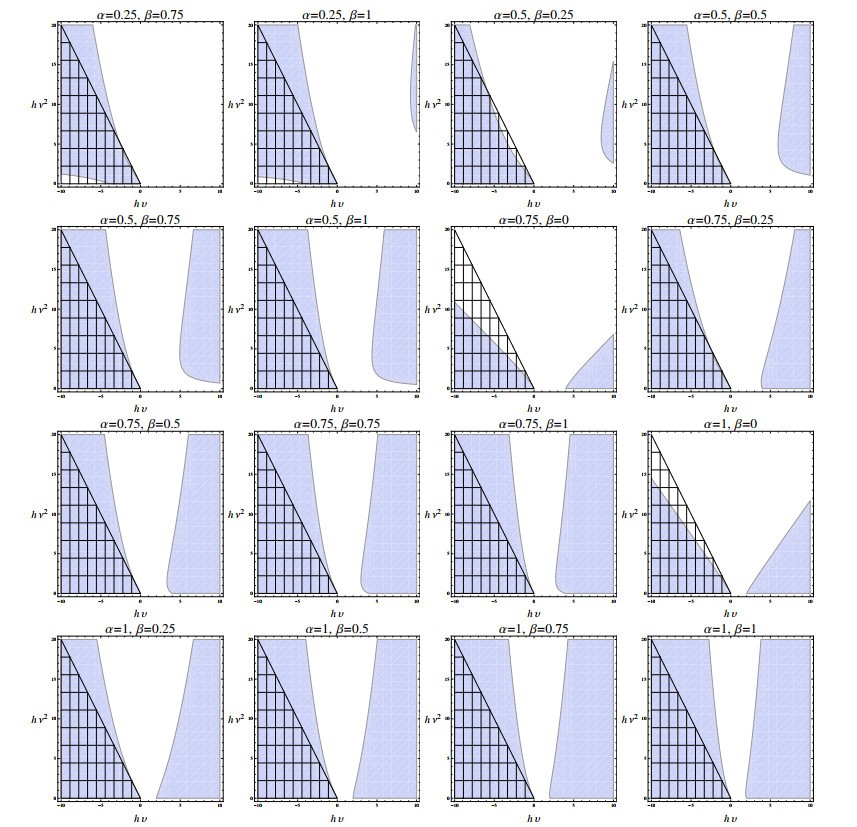
In the present study, we provide a new approximation scheme for solving stochastic differential equations based on the explicit Milstein scheme. Under sufficient conditions, we prove that the split-step $ (\alpha, \beta) $-Milstein scheme strongly convergence to the exact solution with order $ 1.0 $ in mean-square sense. The mean-square stability of our scheme for a linear stochastic differential equation with single and multiplicative commutative noise terms is studied. Stability analysis shows that the mean-square stability of our proposed scheme contains the mean-square stability region of the linear scalar test equation for suitable values of parameters $ \alpha, \beta $. Finally, numerical examples illustrate the effectiveness of the theoretical results.
- Itô stochastic ordinary differential equations,
- mean-square convergence,
- mean-square stability,
- split-step Milstein scheme
Citation: Hassan Ranjbar, Leila Torkzadeh, Dumitru Baleanu, Kazem Nouri. Simulating systems of Itô SDEs with split-step $ (\alpha, \beta) $-Milstein scheme[J]. AIMS Mathematics, 2023, 8(2): 2576-2590. doi: 10.3934/math.2023133

Related Papers:

Abstract

In the present study, we provide a new approximation scheme for solving stochastic differential equations based on the explicit Milstein scheme. Under sufficient conditions, we prove that the split-step $ (\alpha, \beta) $-Milstein scheme strongly convergence to the exact solution with order $ 1.0 $ in mean-square sense. The mean-square stability of our scheme for a linear stochastic differential equation with single and multiplicative commutative noise terms is studied. Stability analysis shows that the mean-square stability of our proposed scheme contains the mean-square stability region of the linear scalar test equation for suitable values of parameters $ \alpha, \beta $. Finally, numerical examples illustrate the effectiveness of the theoretical results.

References

[1]	Z. Korpinar, M. Inc, A. S. Alshomrani, D. Baleanu, The deterministic and stochastic solutions of the Schrödinger equation with time conformable derivative in birefrigent fibers, AIMS Mathematics, 5 (2020), 2326–2345. https://doi.org/10.3934/math.2020154 doi: 10.3934/math.2020154
[2]	K. Nouri, H. Ranjbar, L. Torkzadeh, The explicit approximation approach to solve stiff chemical langevin equations, Eur. Phys. J. Plus, 135 (2020), 758. https://doi.org/10.1140/epjp/s13360-020-00765-2 doi: 10.1140/epjp/s13360-020-00765-2
[3]	K. Nouri, H. Ranjbar, D. Baleanu, L. Torkzadeh, Investigation on ginzburg-landau equation via a tested approach to benchmark stochastic davis-skodje system, Alexandria Eng. J., 60 (2021), 5521–5526. https://doi.org/10.1016/j.aej.2021.04.040 doi: 10.1016/j.aej.2021.04.040
[4]	D. J. Higham, P. E. Kloeden, An introduction to the numerical simulation of stochastic differential equations, Society for Industrial and Applied Mathematics, 2021.
[5]	K. Nouri, F. Fahimi, L. Torkzadeh, D. Baleanu, Stochastic epidemic model of Covid-19 via the reservoir-people transmission network, Comput. Mater. Contin., 72 (2022), 1495–1514. https://doi.org/10.32604/cmc.2022.024406 doi: 10.32604/cmc.2022.024406
[6]	P. E. Kloeden, E. Platen, Numerical solution of stochastic differential equations, In: Applications of mathematics, Berlin: Springer-Verlag, 23 (1992).
[7]	X. Mao, Stochastic differential equations and applications, Chichester: Horwood Publishing Limited, 2008.
[8]	K. Nouri, F. Fahimi, L. Torkzadeh, D. Baleanu, Numerical method for pricing discretely monitored double barrier option by orthogonal projection method, AIMS Mathematics, 6 (2021), 5750–5761. https://doi.org/10.3934/math.2021339 doi: 10.3934/math.2021339
[9]	G. N. Milstein, Approximate integration of stochastic differential equations, Theory Prob. Appl., 19 (1975), 557–562. https://doi.org/10.1137/1119062 doi: 10.1137/1119062
[10]	P. Wang, Z. Liu, Split-step backward balanced Milstein methods for stiff stochastic systems, Appl. Numer. Math., 59 (2009), 1198–1213. https://doi.org/10.1016/j.apnum.2008.06.001 doi: 10.1016/j.apnum.2008.06.001
[11]	D. A. Voss, A. Q. M. Khaliq, Split-step Adams-Moulton Milstein methods for systems of stiff stochastic differential equations, Int. J. Comput. Math., 92 (2015), 995–1011. https://doi.org/10.1080/00207160.2014.915963 doi: 10.1080/00207160.2014.915963
[12]	F. Jiang, X. Zong, C. Yue, C. Huang, Double-implicit and split two-step Milstein schemes for stochastic differential equations, Int. J. Comput. Math., 93 (2016), 1987–2011. https://doi.org/10.1080/00207160.2015.1081182 doi: 10.1080/00207160.2015.1081182
[13]	S. S. Ahmad, N. Chandra Parida, S. Raha, The fully implicit stochastic-$\alpha$ method for stiff stochastic differential equations, J. Comput. Phys., 228 (2009), 8263–8282. https://doi.org/10.1016/j.jcp.2009.08.002 doi: 10.1016/j.jcp.2009.08.002
[14]	V. Reshniak, A. Q. M. Khaliq, D. A. Voss, G. Zhang, Split-step Milstein methods for multi-channel stiff stochastic differential systems, Appl. Numer. Math., 89 (2015), 1–23. https://doi.org/10.1016/j.apnum.2014.10.005 doi: 10.1016/j.apnum.2014.10.005
[15]	T. Tripura, M. Imran, B. Hazra, S. Chakraborty, Change of measure enhanced nearexact euler-maruyama scheme for the solution to nonlinear stochastic dynamical systems, J. Eng. Mech., 148 (2022). http://doi.org/10.1061/(ASCE)EM.1943-7889.0002107
[16]	X. Wang, S. Gan, D. Wang, A family of fully implicit Milstein methods for stiff stochastic differential equations with multiplicative noise, BIT, 52 (2012), 741–772. https://doi.org/10.1007/s10543-012-0370-8 doi: 10.1007/s10543-012-0370-8
[17]	M. S. Semary, M. T. M. Elbarawy, A. F. Fareed, Discrete Temimi-Ansari method for solving a class of stochastic nonlinear differential equations, AIMS Mathematics, 7 (2022), 5093–5105. https://doi.org/10.3934/math.2022283 doi: 10.3934/math.2022283
[18]	J. Yao, S. Gan, Stability of the drift-implicit and double-implicit Milstein schemes for nonlinear SDEs, Appl. Math. Comput., 339 (2018), 294–301. https://doi.org/10.1016/j.amc.2018.07.026 doi: 10.1016/j.amc.2018.07.026
[19]	Z. Yin, S. Gan, An improved Milstein method for stiff stochastic differential equations, Adv. Differ. Equ., 369 (2015). http://doi.org/10.1186/s13662-015-0699-9
[20]	R. Kasinathan, R. Kasinathan, D. Baleanu, A. Annamalai, Well posedness of second-order impulsive fractional neutral stochastic differential equations, AIMS Mathematics, 6 (2021), 9222–9235. https://doi.org/10.3934/math.2021536 doi: 10.3934/math.2021536
[21]	X. Zong, F. Wu, C. Huang, Convergence and stability of the semi-tamed Euler scheme for stochastic differential equations with non-Lipschitz continuous coefficients, Appl. Math. Comput. 228 (2014), 240–250. https://doi.org/10.1016/j.amc.2013.11.100
[22]	Y. Saito, T. Mitsui, Stability analysis of numerical schemes for stochastic differential equations, SIAM J. Numer. Anal., 33 (1996), 2254–2267. https://doi.org/10.1137/S0036142992228409 doi: 10.1137/S0036142992228409
[23]	Y. Saito, T. Mitsui, Mean-square stability of numerical schemes for stochastic differential systems, Vietnam J. Math., 30 (2002), 551–560.
[24]	E. Buckwar, C. Kelly, Towards a systematic linear stability analysis of numerical methods for systems of stochastic differential equations, SIAM J. Numer. Anal., 48 (2010), 298–321. https://doi.org/10.1137/090771843 doi: 10.1137/090771843
[25]	E. Buckwar, T. Sickenberger, A structural analysis of asymptotic mean-square stability for multi-dimensional linear stochastic differential systems, Appl. Numer. Math., 62 (2012), 842–859. https://doi.org/10.1016/j.apnum.2012.03.002 doi: 10.1016/j.apnum.2012.03.002
[26]	D. J. Higham, A-stability and stochastic mean-square stability, BIT, 40 (2000), 404–409. http://doi.org/10.1023/A:1022355410570 doi: 10.1023/A:1022355410570
[27]	A. Tocino, M. J. Senosiain, MS-stability of nonnormal stochastic differential systems, J. Comput. Appl. Math., 379 (2020), 112950. https://doi.org/10.1016/j.cam.2020.112950 doi: 10.1016/j.cam.2020.112950
[28]	D. J. Higham, X. Mao, L. Szpruch, Convergence, non-negativity and stability of a new Milstein scheme with applications to finance, Discrete Contin. Dyn. B, 18 (2013), 2083–2100. https://doi.org/10.3934/dcdsb.2013.18.2083 doi: 10.3934/dcdsb.2013.18.2083
[29]	X. Zong, F. Wu, G. Xu, Convergence and stability of two classes of theta-Milstein schemes for stochastic differential equations, J. Comput. Appl. Math., 336 (2018), 8–29. https://doi.org/10.1016/j.cam.2017.12.025 doi: 10.1016/j.cam.2017.12.025
[30]	K. Nouri, H. Ranjbar, L. Torkzadeh, Improved Euler-Maruyama method for numerical solution of the Itô stochastic differential systems by composite previous-current-step idea, Mediterr. J. Math., 15 (2018), 140.
[31]	K. Nouri, H. Ranjbar, L. Torkzadeh, Modified stochastic theta methods by ODEs solvers for stochastic differential equations, Commun. Nonlinear Sci. Numer. Simul., 68 (2019), 336–346. https://doi.org/10.1016/j.cnsns.2018.08.013 doi: 10.1016/j.cnsns.2018.08.013
[32]	K. Nouri, H. Ranjbar, L. Torkzadeh, Study on split-step Rosenbrock type method for stiff stochastic differential systems, Int. J. Comput. Math., 97 (2020), 816–836. https://doi.org/10.1080/00207160.2019.1589459 doi: 10.1080/00207160.2019.1589459
[33]	G. N. Milstein, M. V. Tretyakov, Stochastic numerics for mathematical physics, Berlin: Springer-Verlag, 2004.
[34]	S. Singh, S. Raha, Five-stage milstein methods for SDEs, Int. J. Comput. Math., 89 (2012), 760–779. http://doi.org/10.1080/00207160.2012.657629 doi: 10.1080/00207160.2012.657629

Reader Comments

Your name:*

Email:*
© 2023 the Author(s), licensee AIMS Press. This is an open access article distributed under the terms of the Creative Commons Attribution License (http://creativecommons.org/licenses/by/4.0)