Recently, there has been increased interest in emotion recognition. It is widely utilised in many industries, including healthcare, education and human-computer interaction (HCI). Different emotions are frequently recognised using characteristics of human emotion. Multimodal emotion identification based on the fusion of several features is currently the subject of increasing amounts of research. In order to obtain a superior classification performance, this work offers a deep learning model for multimodal emotion identification based on the fusion of electroencephalogram (EEG) signals and facial expressions. First, the face features from the facial expressions are extracted using a pre-trained convolution neural network (CNN). In this article, we employ CNNs to acquire spatial features from the original EEG signals. These CNNs use both regional and global convolution kernels to learn the characteristics of the left and right hemisphere channels as well as all EEG channels. Exponential canonical correlation analysis (ECCA) is used to combine highly correlated data from facial video frames and EEG after extraction. The 1-D CNN classifier uses these combined features to identify emotions. In order to assess the effectiveness of the suggested model, this research ran tests on the DEAP dataset. It is found that Multi_Modal_1D-CNN achieves 98.9% of accuracy, 93.2% of precision, 89.3% of recall, 94.23% of F1-score and 7sec of processing time.
Citation: Youseef Alotaibi, Veera Ankalu. Vuyyuru. Electroencephalogram based face emotion recognition using multimodal fusion and 1-D convolution neural network (ID-CNN) classifier[J]. AIMS Mathematics, 2023, 8(10): 22984-23002. doi: 10.3934/math.20231169
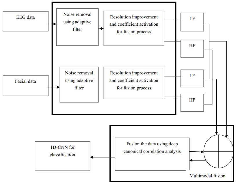
Recently, there has been increased interest in emotion recognition. It is widely utilised in many industries, including healthcare, education and human-computer interaction (HCI). Different emotions are frequently recognised using characteristics of human emotion. Multimodal emotion identification based on the fusion of several features is currently the subject of increasing amounts of research. In order to obtain a superior classification performance, this work offers a deep learning model for multimodal emotion identification based on the fusion of electroencephalogram (EEG) signals and facial expressions. First, the face features from the facial expressions are extracted using a pre-trained convolution neural network (CNN). In this article, we employ CNNs to acquire spatial features from the original EEG signals. These CNNs use both regional and global convolution kernels to learn the characteristics of the left and right hemisphere channels as well as all EEG channels. Exponential canonical correlation analysis (ECCA) is used to combine highly correlated data from facial video frames and EEG after extraction. The 1-D CNN classifier uses these combined features to identify emotions. In order to assess the effectiveness of the suggested model, this research ran tests on the DEAP dataset. It is found that Multi_Modal_1D-CNN achieves 98.9% of accuracy, 93.2% of precision, 89.3% of recall, 94.23% of F1-score and 7sec of processing time.

| [1] |
J. Zhao, X. Mao, L. Chen, Speech emotion recognition using deep 1D & 2D CNN LSTM networks, Biomed. Signal Process. Control, 47 (2019), 312–323. https://doi.org/10.1016/j.bspc.2018.08.035 doi: 10.1016/j.bspc.2018.08.035

|
| [2] |
M. Liu, J. Tang, Audio and video bimodal emotion recognition in social networks based on improved alexnet network and attention mechanism, J. Inf. Process. Syst., 17 (2021), 754–771. https://doi.org/10.3745/JIPS.02.0161 doi: 10.3745/JIPS.02.0161
|
| [3] |
J. N. Njoku, A. C. Caliwag, W. Lim, S. Kim, H. Hwang, J. Jung, Deep learning based data fusion methods for multimodal emotion recognition, J. Korean Inst. Commun. Inf. Sci., 47 (2022), 79–87. https://doi.org/10.7840/kics.2022.47.1.79 doi: 10.7840/kics.2022.47.1.79
|
| [4] |
Q. Ji, Z. Zhu, P. Lan, Real-time nonintrusive monitoring and prediction of driver fatigue, IEEE T. Veh. Techol., 53 (2004), 1052–1068. https://doi.org/10.1109/TVT.2004.830974 doi: 10.1109/TVT.2004.830974
|
| [5] |
H. Zhao, Z. Wang, S. Qiu, J. Wang, F. Xu, Z. Wang, et al., Adaptive gait detection based on foot-mounted inertial sensors and multi-sensor fusion, Inf. Fusion, 52 (2019), 157–166. https://doi.org/10.1016/j.inffus.2019.03.002 doi: 10.1016/j.inffus.2019.03.002
|
| [6] |
J. Gratch, S. Marsella, Evaluating a computational model of emotion, Auton. Agent. Multi-Agent Syst., 11 (2005), 23–43. https://doi.org/10.1007/s10458-005-1081-1 doi: 10.1007/s10458-005-1081-1
|
| [7] |
J. Edwards, H. J. Jackson, P. E. Pattison, Emotion recognition via facial expression and affective prosody in schizophrenia: A methodological review, Clin. Psychol. Rev., 22 (2002), 789–832. https://doi.org/10.1016/S0272-7358(02)00130-7 doi: 10.1016/S0272-7358(02)00130-7
|
| [8] |
T. Fong, I. Nourbakhsh, K. Dautenhahn, A survey of socially interactive robots, Rob. Auton. Syst., 42 (2003), 143–166. https://doi.org/10.1016/S0921-8890(02)00372-X doi: 10.1016/S0921-8890(02)00372-X
|
| [9] |
J.A. Russell, A circumplex model of affect, J. Per. Soc. Psychol., 39 (1980), 1161–1178. https://doi.org/10.1037/h0077714 doi: 10.1037/h0077714
|
| [10] | H. Gunes, B. Schuller, M. Pantic, R. Cowie, Emotion representation, analysis and synthesis in continuous space: A survey, In: 2011 IEEE International Conference on Automatic Face & Gesture Recognition (FG), 2011,827–834. https://doi.org/10.1109/FG.2011.5771357 |
| [11] |
R. Plutchik, The nature of emotions: Human emotions have deep evolutionary roots, a fact that may explain their complexity and provide tools for clinical practice, Am. Sci., 89 (2001), 344–350. http://www.jstor.org/stable/27857503 doi: 10.1511/2001.28.344
|
| [12] | A. Gudi, H. E. Tasli, T. M. Den Uyl, A. Maroulis, Deep learning based facs action unit occurrence and intensity estimation, In: 2015 11th IEEE International Conference and Workshops on Automatic Face and Gesture Recognition (FG), 2015, 1–5. https://doi.org/10.1109/FG.2015.7284873 |
| [13] | R. T. Ionescu, M. Popescu, C. Grozea, Local learning to improve bag of visual words model for facial expression recognition, In: ICML 2013 Workshop on Representation Learning, 2013. |
| [14] |
S. Li, W. Deng, Deep facial expression recognition: A survey, IEEE T. Affect. Comput., 13 (2020), 1195–1215. https://doi.org/10.1109/TAFFC.2020.2981446 doi: 10.1109/TAFFC.2020.2981446
|
| [15] |
S. Wang, J. Qu, Y. Zhang, Y. Zhang, Multimodal emotion recognition from EEG signals and facial expressions, IEEE Access, 11 (2023), 33061–33068. https://doi.org/10.1109/ACCESS.2023.3263670 doi: 10.1109/ACCESS.2023.3263670
|
| [16] |
Y. Jiang, S. Xie, X. Xie, Y. Cui, H. Tang, Emotion recognition via multi-scale feature fusion network and attention mechanism, IEEE Sens. J., 10 (2023), 10790–10800. https://doi.org/10.1109/JSEN.2023.3265688 doi: 10.1109/JSEN.2023.3265688
|
| [17] |
Q. Zhang, H. Zhang, K. Zhou, L. Zhang, Developing a physiological signal-based, mean threshold and decision-level fusion algorithm (PMD) for emotion recognition, Tsinghua. Sci. Techol., 28 (2023), 673–685. https://doi.org/10.26599/TST.2022.9010038 doi: 10.26599/TST.2022.9010038
|
| [18] |
Y. Wang, S. Qiu, D. Li, C. Du, B. L. Lu, H. He, Multi-modal domain adaptation variational autoencoder for eeg-based emotion recognition, IEEE/CAA J. Autom. Sinica, 9 (2022), 1612–1626. https://doi.org/10.1109/JAS.2022.105515 doi: 10.1109/JAS.2022.105515
|
| [19] |
D. Li, J. Liu, Y. Yang, F. Hou, H. Song, Y. Song, et al., Emotion recognition of subjects with hearing impairment based on fusion of facial expression and EEG topographic map, IEEE T. Neur. Syst. Reh., 31 (2022), 437–445. https://doi.org/10.1109/TNSRE.2022.3225948 doi: 10.1109/TNSRE.2022.3225948
|
| [20] |
Y. Wu, J. Li, Multi-modal emotion identification fusing facial expression and EEG, Multimed. Tools Appl., 82 (2023), 10901–10919. https://doi.org/10.1007/s11042-022-13711-4 doi: 10.1007/s11042-022-13711-4
|
| [21] |
D. Y. Choi, D. H. Kim, B. C. Song, Multimodal attention network for continuous-time emotion recognition using video and EEG signals, IEEE Access, 8 (2020), 203814–203826. https://doi.org/10.1109/ACCESS.2020.3036877 doi: 10.1109/ACCESS.2020.3036877
|
| [22] |
E. S. Salama, R. A. El-Khoribi, M. E. Shoman, M. A. W. Shalaby, A 3D-convolutional neural network framework with ensemble learning techniques for multi-modal emotion recognition, Egypt. Inf. J., 22 (2021), 167–176. https://doi.org/10.1016/j.eij.2020.07.005 doi: 10.1016/j.eij.2020.07.005
|
| [23] |
S. Liu, Y. Zhao, Y. An, J. Zhao, S. H. Wang, J. Yan, GLFANet: A global to local feature aggregation network for EEG emotion recognition, Bio. Signal. Process. Control, 85 (2023), 104799. https://doi.org/10.1016/j.bspc.2023.104799 doi: 10.1016/j.bspc.2023.104799
|
| [24] |
Y. Hu, F. Wang, Multi-modal emotion recognition combining face image and EEG signal, J. Circuit. Syst. Comput., 32 (2022), 2350125. https://doi.org/10.1142/S0218126623501256 doi: 10.1142/S0218126623501256
|
| [25] |
S. Liu, Z. Wang, Y. An, J. Zhao, Y. Zhao, Y. D. Zhang, EEG emotion recognition based on the attention mechanism and pre-trained convolution capsule network, Knowl. Based Syst., 265 (2023), 110372. https://doi.org/10.1016/j.knosys.2023.110372 doi: 10.1016/j.knosys.2023.110372
|
| [26] |
C. Li, B. Wang, S. Zhang, Y. Liu, R. Song, J. Cheng, et al., Emotion recognition from EEG based on multi-task learning with capsule network and attention mechanism, Comput. Bio. Med., 143 (2022), 105303. https://doi.org/10.1016/j.compbiomed.2022.105303 doi: 10.1016/j.compbiomed.2022.105303
|
| [27] | S. J. Savitha, M. Paulraj, K. Saranya, Emotional classification using EEG signals and facial expression: A survey, In: Deep Learning Approaches to Cloud Security, Beverly: Scrivener Publishing, 2021, 27–42. https://doi.org/10.1002/9781119760542.ch3 |
| [28] |
Y. Alotaibi, A new meta-heuristics data clustering algorithm based on tabu search and adaptive search memory. Symmetry, 14 (2022), 623. https://doi.org/10.3390/sym14030623 doi: 10.3390/sym14030623
|
| [29] |
H. S. Gill, O. I. Khalaf, Y. Alotaibi, S. Alghamdi, F. Alassery, Multi-model CNN-RNN-LSTM based fruit recognition and classification, Intell. Autom. Soft Comput., 33 (2022), 637–650. https://doi.org/10.32604/iasc.2022.02258 doi: 10.32604/iasc.2022.022589
|
| [30] |
Y. Alotaibi, M. N. Malik, H. H. Khan, A. Batool, S. U. Islam, A. Alsufyani, et al., Suggestion mining from opinionated text of big social media data, CMC, 68 (2021), 3323–3338. https://doi.org/10.32604/cmc.2021.016727 doi: 10.32604/cmc.2021.016727
|
| [31] |
H. S. Gill, O. I. Khalaf, Y. Alotaibi, S. Alghamdi, F. Alassery, Fruit image classification using deep learning, CMC, 71 (2022), 5135–5150. https://doi.org/10.32604/cmc.2022.022809 doi: 10.32604/cmc.2022.022809
|
| [32] |
T. Thanarajan, Y. Alotaibi, S. Rajendran, K. Nagappan, Improved wolf swarm optimization with deep-learning-based movement analysis and self-regulated human activity recognition, AIMS Mathematics, 8 (2023), 12520–12539. https://doi.org/10.3934/math.2023629 doi: 10.3934/math.2023629
|
| [33] |
S. Koelstra, C. Mühl, M. Soleymani, J. S. Lee, A. Yazdani, T. Ebrahimi, et al., DEAP: A database for emotion analysis; using physiological signals, IEEE T. Affect. Comput., 3 (2012), 18–31. https://doi.org/10.1109/T-AFFC.2011.15 doi: 10.1109/T-AFFC.2011.15
|


Figures(8) / Tables(3)

Youseef Alotaibi, Veera Ankalu. Vuyyuru. Electroencephalogram based face emotion recognition using multimodal fusion and 1-D convolution neural network (ID-CNN) classifier[J]. AIMS Mathematics, 2023, 8(10): 22984-23002. doi: 10.3934/math.20231169


 DownLoad: