In clinical diagnostics, magnetic resonance imaging (MRI) technology plays a crucial role in the recognition of cardiac regions, serving as a pivotal tool to assist physicians in diagnosing cardiac diseases. Despite the notable success of convolutional neural networks (CNNs) in cardiac MRI segmentation, it remains a challenge to use existing CNNs-based methods to deal with fuzzy information in cardiac MRI. Therefore, we proposed a novel network architecture named DAFNet to comprehensively address these challenges.
The proposed method was used to design a fuzzy convolutional module, which could improve the feature extraction performance of the network by utilizing fuzzy information that was easily ignored in medical images while retaining the advantage of attention mechanism. Then, a multi-scale feature refinement structure was designed in the decoder portion to solve the problem that the decoder structure of the existing network had poor results in obtaining the final segmentation mask. This structure further improved the performance of the network by aggregating segmentation results from multi-scale feature maps. Additionally, we introduced the dynamic convolution theory, which could further increase the pixel segmentation accuracy of the network.
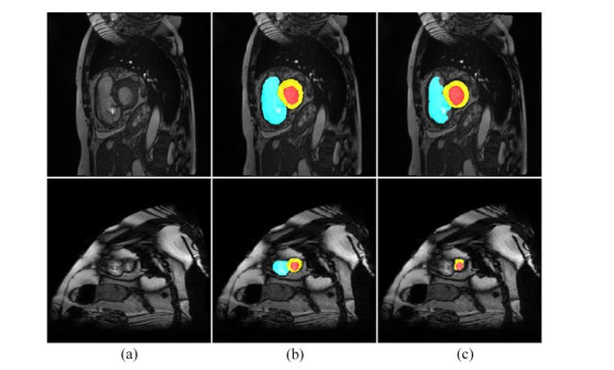
The effectiveness of DAFNet was extensively validated for three datasets. The results demonstrated that the proposed method achieved DSC metrics of 0.942 and 0.885, and HD metricd of 2.50mm and 3.79mm on the first and second dataset, respectively. The recognition accuracy of left ventricular end-diastolic diameter recognition on the third dataset was 98.42%.
Compared with the existing CNNs-based methods, the DAFNet achieved state-of-the-art segmentation performance and verified its effectiveness in clinical diagnosis.
Citation: Yuxin Luo, Yu Fang, Guofei Zeng, Yibin Lu, Li Du, Lisha Nie, Pu-Yeh Wu, Dechuan Zhang, Longling Fan. DAFNet: A dual attention-guided fuzzy network for cardiac MRI segmentation[J]. AIMS Mathematics, 2024, 9(4): 8814-8833. doi: 10.3934/math.2024429
In clinical diagnostics, magnetic resonance imaging (MRI) technology plays a crucial role in the recognition of cardiac regions, serving as a pivotal tool to assist physicians in diagnosing cardiac diseases. Despite the notable success of convolutional neural networks (CNNs) in cardiac MRI segmentation, it remains a challenge to use existing CNNs-based methods to deal with fuzzy information in cardiac MRI. Therefore, we proposed a novel network architecture named DAFNet to comprehensively address these challenges.
The proposed method was used to design a fuzzy convolutional module, which could improve the feature extraction performance of the network by utilizing fuzzy information that was easily ignored in medical images while retaining the advantage of attention mechanism. Then, a multi-scale feature refinement structure was designed in the decoder portion to solve the problem that the decoder structure of the existing network had poor results in obtaining the final segmentation mask. This structure further improved the performance of the network by aggregating segmentation results from multi-scale feature maps. Additionally, we introduced the dynamic convolution theory, which could further increase the pixel segmentation accuracy of the network.
The effectiveness of DAFNet was extensively validated for three datasets. The results demonstrated that the proposed method achieved DSC metrics of 0.942 and 0.885, and HD metricd of 2.50mm and 3.79mm on the first and second dataset, respectively. The recognition accuracy of left ventricular end-diastolic diameter recognition on the third dataset was 98.42%.
Compared with the existing CNNs-based methods, the DAFNet achieved state-of-the-art segmentation performance and verified its effectiveness in clinical diagnosis.

| [1] | World health statistics 2022: Monitoring health for the SDGs, Sustainable development goals, Geneva: World Health Organization, 2022. Available from: https://www.who.int/data/gho/publications/world-health-statistics. |
| [2] |
A. F. Frangi, W. J. Niessen, M. A. Viergever, Three-dimensional modeling for functional analysis of cardiac images, a review, IEEE T. Med. Imaging, 20 (2001), 2−5. https://doi.org/10.1109/42.906421 doi: 10.1109/42.906421

|
| [3] |
S. J. Al'Aref, K. Anchouche, G. Singh, P. J. Slomka, K. K. Kolli, A. Kumar, et al., Clinical applications of machine learning in cardiovascular disease and its relevance to cardiac imaging, Eur. Heart J., 40 (2019), 1975−1986. https://doi.org/10.1093/eurheartj/ehy404 doi: 10.1093/eurheartj/ehy404
|
| [4] | G. I. Sanchez-Ortiz, A. Noble, Fuzzy clustering driven anisotropic diffusion: Enhancement and segmentation of cardiac MR images, In: 1998 IEEE Nuclear Science Symposium Conference Record, IEEE Nuclear Science Symposium and Medical Imaging Conference, 1998, 1873−1874. https://doi.org/10.1109/NSSMIC.1998.773901 |
| [5] |
N. Paragios. A level set approach for shape-driven segmentation and tracking of the left ventricle, IEEE T. Med. Imaging, 22 (2003), 773−776. https://doi.org/10.1109/TMI.2003.814785 doi: 10.1109/TMI.2003.814785
|
| [6] | P. Tran, A fully convolutional neural network for cardiac segmentation in short-axis MRI, arXiv preprint, 2016. Available from: https://arXiv.org/abs/1604.00494. |
| [7] |
E. Shelhamer, J. Long, T. Darrell, Fully convolutional networks for semantic segmentation, IEEE T. Pattern Anal., 39 (2017), 3431−3440. https://doi.org/10.1109/TPAMI.2016.2572683 doi: 10.1109/TPAMI.2016.2572683
|
| [8] |
M. Khened, V. Kollerathu, G. Krishnamurthi, Fully convolutional multi-scale residual DenseNets for cardiac segmentation and automated cardiac diagnosis using ensemble of classifiers, Med. Image Anal., 51 (2019), 21−45. https://doi.org/10.1016/j.media.2018.10.004 doi: 10.1016/j.media.2018.10.004
|
| [9] | O. Ronneberger, P. Fischer, T. Brox, U-net: Convolutional networks for biomedical image segmentation, In: Medical Image Computing and Computer-Assisted Intervention-MICCAI 2015: 18th International Conference, 2015,234−241. https://doi.org/10.1007/978-3-319-24574-4_28 |
| [10] |
N. Painchaud, Y. Skandarani, T. Judge, O. Bernard, A. Lalande, P. M. Jodoin, Cardiac segmentation with strong anatomical guarantees, IEEE T. Med. Imaging, 39 (2020), 3703−3713. https://doi.org/10.1109/TMI.2020.3003240 doi: 10.1109/TMI.2020.3003240
|
| [11] | F. Cheng, C. Chen, Y. Wang, H. Shi, Y. Cao, D. Tu, et al., Learning directional feature maps for cardiac MRI segmentation, In: Medical Image Computing and Computer Assisted Intervention–MICCAI 2020: 23rd International Conference, 2020,108−117. https://doi.org/10.1007/978-3-030-59719-1_11 |
| [12] |
Q. Tong, C. Li, W. Si, X. Liao, Y. Tong, Z. Yuan, et al., RIANet: Recurrent interleaved attention network for cardiac MRI segmentation, Comput. Biol. Med., 109 (2019), 290−302. https://doi.org/10.1016/j.compbiomed.2019.04.042 doi: 10.1016/j.compbiomed.2019.04.042
|
| [13] |
W. Wang, Q. Xia, Z. Hu, Z. Yan, Z. Li, Y. Wu, et al., Few-shot learning by a cascaded framework with shape-constrained pseudo label assessment for whole heart segmentation, IEEE T. Med. Imaging, 40 (2021), 2629−2641. https://doi.org/10.1109/TMI.2021.3053008 doi: 10.1109/TMI.2021.3053008
|
| [14] | Y. Gao, M. Zhou, D. N. Metaxas, UTNet: A hybrid transformer architecture for medical image segmentation, In: Medical Image Computing and Computer Assisted Intervention, 2021, 61−71. https://doi.org/10.1007/978-3-030-87199-4_6 |
| [15] | A. Rahman, J. Valanarasu, I. Hacihaliloglu, V. M. Patel, Ambiguous medical image segmentation using diffusion models, In: IEEE/CVF Conference on Computer Vision and Pattern Recognition, 2023, 11536−11546. https://doi.org/10.1109/CVPR52729.2023.01110 |
| [16] |
J. Schlemper, O. Oktay, M. Schaap, M. Heinrich, B. Kainz, B. Glocker, et al., Attention gated networks: Learning to leverage salient regions in medical images, Med. Image Anal., 53 (2019), 197−207. https://doi.org/10.1016/j.media.2019.01.012 doi: 10.1016/j.media.2019.01.012
|
| [17] |
J. Hu, L. Shen, G. Sun, Squeeze-and-excitation networks, IEEE T. Pattern Anal., 42 (2020), 2011−2023. https://doi.org/10.1109/TPAMI.2019.2913372 doi: 10.1109/TPAMI.2019.2913372
|
| [18] | S. Woo, J. Park, J. Y. Lee, I. S. Kweon, Cbam: Convolutional block attention module, In: European Conference on Computer Vision-ECCV 2018, Lecture Notes in Computer Science, 2018, 11211. https://doi.org/10.1007/978-3-030-01234-2_1 |
| [19] | Y. Chen, X. Dai, M. Liu, D. Chen, L. Yuan, Z. Liu, Dynamic convolution: Attention over convolution kernels, In: 2020 IEEE/CVF Conference on Computer Vision and Pattern Recognition, 2020, 11027−11036. https://doi.org/10.1109/CVPR42600.2020.01104 |
| [20] |
O. Bernard, A. Lalande, C. Zotti, F. Cervenansky, X. Yang, P. A. Heng, et al., Deep learning techniques for automatic MRI cardiac multi-structures segmentation and diagnosis: Is the problem solved? IEEE T. Med. Imaging, 37 (2018), 2514−2525. https://doi.org/10.1109/TMI.2018.2837502 doi: 10.1109/TMI.2018.2837502
|
| [21] |
V. Campello, P. Gkontra; C. Izquierdo, C. Martin-Isla, A. Sojoudi, P. M. Full, et al., Multi-centre, multi-vendor and multi-disease cardiac segmentation: The M&Ms challenge, IEEE T. Med. Imaging, 12 (2021), 3543−3554. https://doi.org/10.1109/TMI.2021.3090082 doi: 10.1109/TMI.2021.3090082
|
| [22] | T. Lin, P. Dollar, R. Girshick, K. He, B. Hariharan, S. Belongie, Feature pyramid networks for object detection, In: IEEE Conference on Computer Vision and Pattern Recognition, 2017, 2117−2125. https://doi.org/10.1109/CVPR.2017.106 |
| [23] | Y. Ioannou, D. Robertson, R. Cipolla, A. Criminisi, Deep roots: Improving CNN efficiency with hierarchical filter groups, In: 2017 IEEE Conference on Computer Vision and Pattern Recognition, 2017, 1231−1240. https://doi.org/10.1109/CVPR.2017.633 |
| [24] |
A. Ammari, R. Mahmoudi, B. Hmida, R. Saouli, M. H. Bedoui, A review of approaches investigated for right ventricular segmentation using short-axis cardiac MRI, IET Image Process., 15 (2021), 1845−1868. https://doi.org/10.1049/ipr2.12165 doi: 10.1049/ipr2.12165
|
| [25] | K. He, X. Zhang, S. Ren, J. Sun, Deep residual learning for image recognition, In: 2016 IEEE Conference on Computer Vision and Pattern Recognition, 2016,770−778. https://doi.org/10.1109/CVPR.2016.90 |
| [26] |
G. Simantiris, G. Tziritas, Cardiac MRI segmentation with a dilated CNN incorporating domainspecific constraints, IEEE J.-STSP, 14 (2020), 1235−1243. https://doi.org/10.1109/JSTSP.2020.3013351 doi: 10.1109/JSTSP.2020.3013351
|
| [27] | J. M. Wolterink, T. Leiner, M. A. Viergever, I. Išgum, Automatic segmentation and disease classification using cardiac cine MR images, In: Statistical Atlases and Computational Models of the Heart & ACDC and MMWHS Challenges, 2017, 1235−1243. https://doi.org/10.1007/978-3-319-75541-0_11 |
| [28] | C. Baumgartner, L. Koch, M. Pollefeys, E. Konukoglu, An exploration of 2D and 3D deep learning techniques for cardiac MR image segmentation, In: Statistical Atlases and Computational Models the Heart & ACDC and MMWHS Challenges, 2018,111−119. https://doi.org/10.1007/978-3-319-75541-0_12 |
| [29] | F. Isensee, P. F. Jaeger, P. M. Full, I. Wolf, S. Engelhardt, K. H. Maier-Hein, Automatic cardiac disease assessment on cine-MRI via time-series segmentation and domain specific features, In: Statistical Atlases and Computational Models of the Heart, ACDC and MMWHS Challenges, 2018,120−129. https://doi.org/10.1007/978-3-319-75541-0_13 |
| [30] | P. Full, F. Isensee, P. Jager, K. Maier-Hein, Studying robustness of semantic segmentation under domain shift in cardiac MRI, In: Statistical Atlases and Computational Models of the Heart, M&Ms and EMIDEC Challenges, 2021,238−249. https://doi.org/10.1007/978-3-030-68107-4_24 |
| [31] | Y. Zhang, J. Yang, F. Hou, Y. Liu, Y. Wang, J. Tian, et al., Semi-supervised cardiac image segmentation via label propagation and style transfer, In: Statistical Atlases and Computational Models of the Heart, M&Ms and EMIDEC Challenges, 2021,219−227. https://doi.org/10.1007/978-3-030-68107-4_22 |
| [32] | J. Ma, Histogram matching augmentation for domain adaptation with application to multi-centre, multi-vendor and multi-disease cardiac image segmentation, In: Statistical Atlases and Computational Models of the Heart, M&Ms and EMIDEC Challenges, 2021,177−186. https://doi.org/10.1007/978-3-030-68107-4_18 |
| [33] |
F. Isensee, P. Jaeger, S. Kohl, J. Petersen, K. H. Maier-Hein, nnU-Net: A self-configuring method for deep learning-based biomedical image segmentation, Nat. Methods, 18 (2021), 203−211. https://doi.org/10.1038/s41592-020-01008-z doi: 10.1038/s41592-020-01008-z
|
| [34] |
M. Forouzanfar, N. Forghani, M. Teshnehlab, Parameter optimization of improved fuzzy c-means clustering algorithm for brain MR image segmentation, Eng. Appl. Artif. Intel., 23 (2010), 160−168. https://doi.org/10.1016/j.engappai.2009.10.002 doi: 10.1016/j.engappai.2009.10.002
|
| [35] |
N. Tajbakhsh, J. Shin; R. Suryakanth, R. T. Hurst, C. B. Kendall, M. B. Gotway, et al., Convolutional neural networks for medical image analysis: Full training or fine tuning? IEEE T. Med. Imaging, 35 (2016), 1299−1312. https://doi.org/10.1109/TMI.2016.2535302 doi: 10.1109/TMI.2016.2535302
|
| [36] |
T. Lossau, H. Nickisch, T. Wissel, M. Morlock, M. Grass, Learning metal artifact reduction in cardiac CT images with moving pacemakers, Med. Image Anal., 61 (2020), 101655. https://doi.org/10.1016/j.media.2020.101655 doi: 10.1016/j.media.2020.101655
|


Figures(12) / Tables(8)

Yuxin Luo, Yu Fang, Guofei Zeng, Yibin Lu, Li Du, Lisha Nie, Pu-Yeh Wu, Dechuan Zhang, Longling Fan. DAFNet: A dual attention-guided fuzzy network for cardiac MRI segmentation[J]. AIMS Mathematics, 2024, 9(4): 8814-8833. doi: 10.3934/math.2024429


 DownLoad: