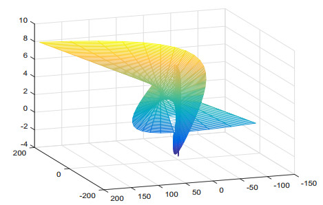
In this paper, we give the existence and uniqueness theorems for non-lightlike framed surfaces and define a special non-lightlike ruled surface in Minkowski 3-space. It may have singularities. We give the conditions for identifying cross-caps and surfaces as developable and maximal. Besides, we demonstrate that if the spacelike ruled surface is developable, then the $ z $-parameter curve is an asymptotic curve if and only if the ruled surface is maximal.
Citation: Chang Sun, Kaixin Yao, Donghe Pei. Special non-lightlike ruled surfaces in Minkowski 3-space[J]. AIMS Mathematics, 2023, 8(11): 26600-26613. doi: 10.3934/math.20231360
In this paper, we give the existence and uniqueness theorems for non-lightlike framed surfaces and define a special non-lightlike ruled surface in Minkowski 3-space. It may have singularities. We give the conditions for identifying cross-caps and surfaces as developable and maximal. Besides, we demonstrate that if the spacelike ruled surface is developable, then the $ z $-parameter curve is an asymptotic curve if and only if the ruled surface is maximal.

| [1] | M. Emmer, Imagine math, Milano: Springer, 2012. https://doi.org/10.1007/978-88-470-2427-4 |
| [2] |
O. Kaya, M. Önder, Generalized normal ruled surface of a curve in the Euclidean 3-space, Acta U. Sapientiae-Ma., 13 (2021), 217–238. https://doi.org/10.2478/ausm-2021-0013 doi: 10.2478/ausm-2021-0013

|
| [3] | O. Kaya, T. Kahraman, M. Önder, Osculating-type ruled surfaces in the Euclidean 3-space, Facta Univ-Ser. Math., 36 (2021), 939–959. |
| [4] | M. Önder, T. Kahraman, On rectifying ruled surfaces, Kuwait J. Sci., 47 (2020), 1–11. |
| [5] |
S. Honda, M. Takahashi, Framed curves in the Euclidean space, Adv. Geom., 16 (2016), 265–276. https://doi.org/10.1515/advgeom-2015-0035 doi: 10.1515/advgeom-2015-0035
|
| [6] |
Ö. G. Yıldız, M. Akyiğit, M. Tosun, On the trajectory ruled surfaces of framed base curves in the Euclidean space, Math. Meth. Appl. Sci., 44 (2021), 7463–7470. https://doi.org/10.1002/mma.6267 doi: 10.1002/mma.6267
|
| [7] |
T. Fukunaga, M. Takahashi, Framed surfaces in the Euclidean space, Bull. Braz. Math. Soc. New Series, 50 (2019), 37–65. https://doi.org/10.1007/s00574-018-0090-z doi: 10.1007/s00574-018-0090-z
|
| [8] |
J. Huang, D. Pei, Singularities of non-developable surfaces in three-dimensional Euclidean space, Mathematics, 7 (2019), 1106. https://doi.org/10.3390/math7111106 doi: 10.3390/math7111106
|
| [9] |
B. D. Yazıcı, Z. Işbilir, M. Tosun, Generalized osculating-type ruled surfaces of singular curves, Math. Meth. Appl. Sci., 46 (2023), 85320–8545. https://doi.org/10.1002/mma.8997 doi: 10.1002/mma.8997
|
| [10] |
K. Eren, Ö. G. Yıldız, M. Akyiğit, Tubular surfaces associated with framed base curves in Euclidean 3-space, Math. Meth. Appl. Sci., 45 (2022), 12110–12118. https://doi.org/10.1002/mma.7590 doi: 10.1002/mma.7590
|
| [11] |
O. Kobayashi, Maximal surfaces in the 3-dimensional Minkowski space ${L}^{3}$, Tokyo J. Math., 6 (1983), 297–309. https://doi.org/10.3836/tjm/1270213872 doi: 10.3836/tjm/1270213872
|
| [12] |
Y. H. Kim, D. W. Yoon, Classification of ruled surfaces in Minkowski 3-spaces, J. Geom. Phys., 49 (2004), 89–100. https://doi.org/10.1016/S0393-0440(03)00084-6 doi: 10.1016/S0393-0440(03)00084-6
|
| [13] | A. T. Vanli, H. H. Hacisalihoglu, On the distribution parameter of timelike ruled surfaces in the Minkowski $3$-space, Far East J. Math. Sci., 5 (1997), 321–328. |
| [14] |
N. Yüksel, The ruled surfaces according to Bishop frame in Minkowski 3-space, Abstr. Appl. Anal., 2013 (2013), 810640. https://doi.org/10.1155/2013/810640 doi: 10.1155/2013/810640
|
| [15] | A. Turgut, H. H. Hacısalihoğlu, Spacelike ruled surfaces in the Minkowski 3-Space, Commun. Fac. Sci. Univ. Ank. Series A1, 46 (1997), 83–91. |
| [16] |
Y. Yayli, S. Saracoglu, On developable ruled surfaces in Minkowski space, Adv. Appl. Clifford Algebras, 22 (2012), 499–510. https://doi.org/10.1007/s00006-011-0305-5 doi: 10.1007/s00006-011-0305-5
|
| [17] |
H. Liu, Ruled surfaces with lightlike ruling in 3-Minkowski space, J. Geom. Phys., 59 (2009), 74–78. https://doi.org/10.1016/j.geomphys.2008.10.003 doi: 10.1016/j.geomphys.2008.10.003
|
| [18] | S. Izumiya, N. Takeuchi, Geometry of ruled surfaces, In: Applicable mathematics in the golden age, New Delhi: Narosa Publishing House, 2003. |
Figures(1)

Chang Sun, Kaixin Yao, Donghe Pei. Special non-lightlike ruled surfaces in Minkowski 3-space[J]. AIMS Mathematics, 2023, 8(11): 26600-26613. doi: 10.3934/math.20231360


 DownLoad: