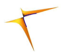
Using a common tangent vector field to a surface along a curve, in this study we discussed a new Darboux frame that we referred to as the rotation-minimizing Darboux frame (RMDF) in Minkowski 3-space. The parametric equation resulting from the RMDF frame for an imbricate-ruled surface was then provided. As a result, minimal (or maximal for timelike surfaces) ruled surfaces were derived, along with the necessary and sufficient criteria for imbricate-ruled surfaces to be developable. The surfaces also described the parameter curves of these surfaces' asymptotic, geodesic, and curvature lines. We also gave an example to emphasize the most significant results.
Citation: Emad Solouma, Ibrahim Al-Dayel, Meraj Ali Khan, Youssef A. A. Lazer. Characterization of imbricate-ruled surfaces via rotation-minimizing Darboux frame in Minkowski 3-space $ \mathrm{E}_1^3 $[J]. AIMS Mathematics, 2024, 9(5): 13028-13042. doi: 10.3934/math.2024635
Using a common tangent vector field to a surface along a curve, in this study we discussed a new Darboux frame that we referred to as the rotation-minimizing Darboux frame (RMDF) in Minkowski 3-space. The parametric equation resulting from the RMDF frame for an imbricate-ruled surface was then provided. As a result, minimal (or maximal for timelike surfaces) ruled surfaces were derived, along with the necessary and sufficient criteria for imbricate-ruled surfaces to be developable. The surfaces also described the parameter curves of these surfaces' asymptotic, geodesic, and curvature lines. We also gave an example to emphasize the most significant results.

| [1] | M. P. Do Carmo, Differential geometry of curves and surfaces: Revised and updated second edition, Courier Dover Publications, 2016. |
| [2] | T. Shifrin, Differential geometry: A first course in curves and surfaces, University of Georgia, Preliminary Version, 2018. |
| [3] |
M. T. Aldossary, R. A. Abdel-Baky, Sweeping surface due to rotation minimizing Darboux frame in Euclidean 3-space $\mathbb{E}^3$, AIMS Math., 8 (2023), 447–462. https://doi.org/10.3934/math.2023021 doi: 10.3934/math.2023021

|
| [4] |
C. Sun, K. Yao, D. Pei, Special non-lightlike ruled surfaces in Minkowski 3-space, AIMS Math., 8 (2023), 26600–26613. https://doi.org/10.3934/math.20231360 doi: 10.3934/math.20231360
|
| [5] |
M. Dede, M. C. Aslan, M. C. Ekici, On a variational problem due to the $B$-Darboux frame in Euclidean 3-space, Math. Method. Appl. Sci., 44 (2021), 12630–12639. https://doi.org/10.1002/mma.7567 doi: 10.1002/mma.7567
|
| [6] |
E. Solouma, M. Abdelkawy, Family of ruled surfaces generated by equiform Bishop spherical image in Minkowski 3-space, AIMS Math., 8 (2023), 4372–4389. https://doi.org/10.3934/math.2023218 doi: 10.3934/math.2023218
|
| [7] | E. Solouma, On geometry of equiform Smarandache ruled surfaces via equiform frame in Minkowski 3-Space, Appl. Appl. Math., 18 (2023), 1. |
| [8] |
E. Solouma, I. Al-Dayel, M. A. Khan, M. Abdelkawy, Investigation of special type-$II$ smarandache ruled surfaces due to rotation minimizing Darboux frame in $E^3$, Symmetry, 15 (2023), 2207. https://doi.org/10.3390/sym15122207 doi: 10.3390/sym15122207
|
| [9] |
F. Mofarreh, Timelike-ruled and developable surfaces in Minkowski 3-Space $\mathbb{E}_1^3$, Front. Phys., 10 (2022), 838957. https://doi.org/10.3389/fphy.2022.838957 doi: 10.3389/fphy.2022.838957
|
| [10] |
I. AL-Dayel, E. Solouma, M. Khan, On geometry of focal surfaces due to B-Darboux and type-2 Bishop frames in Euclidean 3-space, AIMS Math., 7 (2022), 13454–13468. https://doi.org/10.3934/math.2022744 doi: 10.3934/math.2022744
|
| [11] | G. U. Kaymanli, Characterization of the evolute offset of ruled surfaces with $B$-Darboux frame, J. New Theor., 33 (2020), 50–55. |
| [12] | S. Ouarab, A. O. Chahdi, M. Izid, Ruled surface generated by a curve lying on a regular surface and its characterizations, J. Geom. Graph., 24 (2020), 257–267. |
| [13] |
E. M. Solouma, I. AL-Dayel, Harmonic evolute surface of tubular surfaces via $B$-Darboux frame in Euclidean 3-space, Adv. Math. Phys., 2021 (2021), 5269655. https://doi.org/10.1155/2021/5269655 doi: 10.1155/2021/5269655
|
| [14] |
S. Hu, Z. Wang, X. Tang, Tubular surfaces of center curves on spacelike surfaces in Lorentz-Minkowski 3-space, Math. Method. Appl. Sci., 42 (2019), 3136–3166. https://doi.org/10.1002/mma.5574 doi: 10.1002/mma.5574
|
| [15] |
Y. Li, F. Mofarreh. R. A. Abdel-Baky, Timelike circular surfaces and singularities in Minkowski 3-Space, Symmetry, 14 (2022), 1914. https://doi.org/10.3390/sym14091914 doi: 10.3390/sym14091914
|
| [16] |
Y. Li, Z. Chen, S. H. Nazra, R. A. Abdel-Baky, Singularities for timelike developable surfaces in Minkowski 3-Space, Symmetry, 15 (2023), 277. https://doi.org/10.3390/sym15020277 doi: 10.3390/sym15020277
|
| [17] | G. Darboux, Leçons sur la theorie Generale des surfaces, Gauthier-Villars, 1896. |
| [18] | B. O'Neill, Semi-Riemannian geometry with applications to relativity, Academic press, 1983. |
| [19] |
R. López, Differential geometry of curves and surfaces in Lorentz-Minlowski space, Int. Electron. J. Geom., 7 (2014), 44–107. https://doi.org/10.36890/iejg.594497 doi: 10.36890/iejg.594497
|
| [20] |
K. E. Özen, M. Tosun, A new moving frame for trajectories with non-vanishing angular Momentum, J. Math. Sci. Model., 4 (2021), 7–18. https://doi.org/10.33187/jmsm.869698 doi: 10.33187/jmsm.869698
|


Figures(4)

Emad Solouma, Ibrahim Al-Dayel, Meraj Ali Khan, Youssef A. A. Lazer. Characterization of imbricate-ruled surfaces via rotation-minimizing Darboux frame in Minkowski 3-space $ \mathrm{E}_1^3 $[J]. AIMS Mathematics, 2024, 9(5): 13028-13042. doi: 10.3934/math.2024635


 DownLoad: