Codimension-two bifurcation analysis at an endemic equilibrium state of a discrete epidemic model

Abdul Qadeer Khan; Tania Akhtar; Adil Jhangeer; Muhammad Bilal Riaz; Abdul Qadeer Khan; Tania Akhtar; Adil Jhangeer; Muhammad Bilal Riaz

doi:10.3934/math.2024634

AIMS Mathematics

2024, Volume 9, Issue 5: 13006-13027. doi: 10.3934/math.2024634

Previous Article Next Article

Research article

Codimension-two bifurcation analysis at an endemic equilibrium state of a discrete epidemic model

1.
Department of Mathematics, University of Azad Jammu and Kashmir, Muzaffarabad 13100, Pakistan
2.
Department of Mathematics, Namal University, Mianwali, Pakistan
3.
IT4Innovations, VSB-Technical University of Ostrava, Ostrava, Czech Republic
4.
Department of Computer Science and Mathematics, Lebanese American University, Byblos, Lebanon

Received: 20 January 2024 Revised: 04 March 2024 Accepted: 20 March 2024 Published: 07 April 2024
MSC : 40A05, 70K50, 92D25

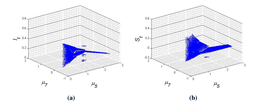
In this paper, we examined the codimension-two bifurcation analysis of a two-dimensional discrete epidemic model. More precisely, we examined the codimension-two bifurcation analysis at an endemic equilibrium state associated with $ 1:2 $, $ 1:3 $ and $ 1:4 $ strong resonances by bifurcation theory and series of affine transformations. Finally, theoretical results were carried out numerically.
- codimension-two bifurcation,
- strong resonances,
- numerical simulation,
- epidemic model,
- affine transformations
Citation: Abdul Qadeer Khan, Tania Akhtar, Adil Jhangeer, Muhammad Bilal Riaz. Codimension-two bifurcation analysis at an endemic equilibrium state of a discrete epidemic model[J]. AIMS Mathematics, 2024, 9(5): 13006-13027. doi: 10.3934/math.2024634

Related Papers:

Abstract

In this paper, we examined the codimension-two bifurcation analysis of a two-dimensional discrete epidemic model. More precisely, we examined the codimension-two bifurcation analysis at an endemic equilibrium state associated with $ 1:2 $, $ 1:3 $ and $ 1:4 $ strong resonances by bifurcation theory and series of affine transformations. Finally, theoretical results were carried out numerically.

References

[1]	J. P. Langa, C. Sema, N. D. Deus, M. M. Colombo, E. Taviani, Epidemic waves of cholera in the last two decades in Mozambique, J. Infect. Dev. Ctries., 9 (2015), 635–641. https://doi.org/10.3855/jidc.6943 doi: 10.3855/jidc.6943
[2]	M. H. Azizi, J. G. A. Raeis, F. Azizi, A history of the 1918 Spanish influenza pandemic and its impact on Iran, Arch. Iran Med., 13 (2010), 262–265.
[3]	C. J. Mussap, The plague doctor of Venice, Intern. Med. J., 49 (2019), 671–676. https://doi.org/10.1111/imj.14285
[4]	W. O. Kermack, A. G. McKendrick, A contribution to the mathematical theory of epidemics, Proc. R. Soc. Lond., 115 (1927), 700–721. https://doi.org/10.1098/rspa.1927.0118 doi: 10.1098/rspa.1927.0118
[5]	A. Q. Khan, M. Tasneem, M. B. Almatrafi, Discrete-time covid-19 epidemic model with bifurcation and control, Math. Biosci. Eng., 19 (2021), 1944–1969. https://doi.org/10.3934/mbe.2022092 doi: 10.3934/mbe.2022092
[6]	M. Pájaro, N. M. Fajar, A. A. Alonso, I. Otero-Muras, Stochastic SIR model predicts the evolution of COVID-19 epidemics from public health and wastewater data in small and medium-sized municipalities: A one year study, Chaos Solit. Fractals, 164 (2022), 112671. https://doi.org/10.1016/j.chaos.2022.112671 doi: 10.1016/j.chaos.2022.112671
[7]	K. Ghosh, A. K. Ghosh, Study of COVID-19 epidemiological evolution in India with a multi-wave SIR model, Nonlinear Dyn., 109 (2022), 47–55. https://doi.org/10.1007/s11071-022-07471-x doi: 10.1007/s11071-022-07471-x
[8]	S. O. Gladkov, On the question of self-organization of population dynamics on earth, Biophysics, 66 (2021), 858–866. https://doi.org/10.1134/S0006350921050055 doi: 10.1134/S0006350921050055
[9]	L. Ma, D. Hu, Z. Zheng, C. Q. Ma, M. Liu, Multiple bifurcations in a mathematical model of glioma-immune interaction, Commun. Nonlinear Sci. Numer. Simul., 123 (2023), 107282. https://doi.org/10.1016/j.cnsns.2023.107282 doi: 10.1016/j.cnsns.2023.107282
[10]	X. Zhang, J. Wu, P. Zhao, X. Su, D. Choi, Epidemic spreading on a complex network with partial immunization, Soft Comput., 22 (2018), 4525–4533. https://doi.org/10.1007/s00500-017-2903-1 doi: 10.1007/s00500-017-2903-1
[11]	H. Garg, A. Nasir, N. Jan, S. U. Khan, Mathematical analysis of COVID-19 pandemic by using the concept of SIR model, Soft Comput., 27 (2023), 3477–3491. https://doi.org/10.1007/s00500-021-06133-1 doi: 10.1007/s00500-021-06133-1
[12]	M. Hossain, S. Garai, S. Jafari, N. Pal, Bifurcation, chaos, multistability, and organized structures in a predator-prey model with vigilance, Chaos, 32 (2022), 063139. https://doi.org/10.1063/5.0086906 doi: 10.1063/5.0086906
[13]	X. Li, W. Wang, A discrete epidemic model with stage structure, Chaos Solit. Fractals, 26 (2005), 947–958. https://doi.org/10.1016/j.chaos.2005.01.063 doi: 10.1016/j.chaos.2005.01.063
[14]	W. Du, J. Zhang, S. Qin, J. Yu, Bifurcation analysis in a discrete SIR epidemic model with the saturated contact rate and vertical transmission, J. Nonlinear Sci. Appl., 9 (2016), 4976–4989. http://dx.doi.org/10.22436/jnsa.009.07.02 doi: 10.22436/jnsa.009.07.02
[15]	M. El-Shahed, I. M. Abdelstar, Stability and bifurcation analysis in a discrete-time SIR epidemic model with fractional-order, Int. J. Nonlinear Sci. Numer. Simul., 20 (2019), 339–350. https://doi.org/10.1515/ijnsns-2018-0088 doi: 10.1515/ijnsns-2018-0088
[16]	S. R. J. Jang, Backward bifurcation in a discrete SIS model with vaccination, J. Biol. Syst., 16 (2008), 479–494. https://doi.org/10.1142/S0218339008002630 doi: 10.1142/S0218339008002630
[17]	D. Hu, H. Cao, Bifurcation and chaos in a discrete-time predator-prey system of Holling and Leslie type, Commun. Nonlinear Sci. Numer. Simul., 22 (2015), 702–715. https://doi.org/10.1016/j.cnsns.2014.09.010 doi: 10.1016/j.cnsns.2014.09.010
[18]	D. M. Morens, G. K. Folkers, A. S. Fauci, The challenge of emerging and re-emerging infectious diseases, Nature, 430 (2004), 242–249.
[19]	L. J. Allen, Some discrete-time SI, SIR, and SIS epidemic models, Math. Biosci., 124 (1994), 83–105. https://doi.org/10.1016/0025-5564(94)90025-6
[20]	X. Y. Meng, T. Zhang, The impact of media on the spatiotemporal pattern dynamics of a reaction-diffusion epidemic model, Math. Biosci. Eng., 17 (2020), 4034–4047. https://doi.org/10.3934/mbe.2020223 doi: 10.3934/mbe.2020223
[21]	Y. Wang, Z. Wei, J. Cao, Epidemic dynamics of influenza-like diseases spreading in complex networks, Nonlinear Dyn., 101 (2020), 1801–1820. https://doi.org/10.1007/s11071-020-05867-1 doi: 10.1007/s11071-020-05867-1
[22]	A. Suryanto, I. Darti, On the nonstandard numerical discretization of SIR epidemic model with a saturated incidence rate and vaccination, AIMS Math., 6 (2021), 141–155. https://doi.org/10.3934/math.2021010 doi: 10.3934/math.2021010
[23]	Y. A. Kuznetsov, H. G. Meijer, Numerical bifurcation analysis of maps, Cambridge University Press, 2019. https://doi.org/10.1017/9781108585804
[24]	W. Govaerts, Y. A. Kuznetsov, R. K. Ghaziani, H. G. E. Meijer, Cl MatContM: A toolbox for continuation and bifurcation of cycles of maps, Netherlands, 2008.
[25]	N. Neirynck, B. Al-Hdaibat, W. Govaerts, Y. A. Kuznetsov, H. G. Meijer, Using MatContM in the study of a nonlinear map in economics, J. Phys. Conf. Ser., 692 (2016), 012013. https://doi.org/10.1088/1742-6596/692/1/012013 doi: 10.1088/1742-6596/692/1/012013
[26]	W. Govaerts, R. K. Ghaziani, Y. A. Kuznetsov, H. G. Meijer, Numerical methods for two-parameter local bifurcation analysis of maps, SIAM J. Sci. Comput., 29 (2007), 2644–2667. https://doi.org/10.1137/060653858 doi: 10.1137/060653858
[27]	S. Ruan, W. Wang, Dynamical behavior of an epidemic model with a nonlinear incidence rate, J. Differ. Equ., 188 (2003), 135–163. https://doi.org/10.1016/S0022-0396(02)00089-X doi: 10.1016/S0022-0396(02)00089-X
[28]	Z. Eskandari, J. Alidousti, Stability and codimension 2 bifurcations of a discrete time SIR model, J. Frank. Inst., 357 (2020), 10937–10959. https://doi.org/10.1016/j.jfranklin.2020.08.040 doi: 10.1016/j.jfranklin.2020.08.040
[29]	M. Ruan, C. Li, X. Li, Codimension two 1:1 strong resonance bifurcation in a discrete predator-prey model with Holling IV functional response, AIMS Math., 7 (2021), 3150–3168. https://doi.org/10.3934/math.2022174 doi: 10.3934/math.2022174
[30]	M. A. Abdelaziz, A. I. Ismail, F. A. Abdullah, M. H. Mohd, Codimension-one and two bifurcations of a discrete-time fractional-order SEIR measles epidemic model with constant vaccination, Chaos Solit. Fractals, 140 (2020), 110104. https://doi.org/10.1016/j.chaos.2020.110104 doi: 10.1016/j.chaos.2020.110104
[31]	Q. Chen, Z. Teng, L. Wang, H. Jiang, The existence of codimension-two bifurcation in a discrete SIS epidemic model with standard incidence, Nonlinear Dyn., 71 (2013), 55–73. https://doi.org/10.1007/s11071-012-0641-6 doi: 10.1007/s11071-012-0641-6
[32]	X. Liu, P. Liu, Y. Liu, The existence of codimension-two bifurcations in a discrete-time SIR epidemic model, AIMS Math., 7 (2022), 3360–3379. https://doi.org/10.3934/math.2022187 doi: 10.3934/math.2022187
[33]	N. Yi, Q. Zhang, P. Liu, Y. Lin, Codimension-two bifurcations analysis and tracking control on a discrete epidemic model, J. Syst. Sci. Complex., 24 (2011), 1033–1056. https://doi.org/10.1007/s11424-011-9041-0 doi: 10.1007/s11424-011-9041-0
[34]	J. Ma, M. Duan, Codimension-two bifurcations of a two-dimensional discrete time Lotka-Volterra predator-prey model, Discrete Contin. Dyn. Syst. B, 29 (2024), 1217–1242. https://doi.org/10.3934/dcdsb.2023131 doi: 10.3934/dcdsb.2023131
[35]	A. M. Yousef, A. M. Algelany, A. A. Elsadany, Codimension-one and codimension-two bifurcations in a discrete Kolmogorov type predator-prey model, J. Comput. Appl. Math., 428 (2023), 115171. https://doi.org/10.1016/j.cam.2023.115171 doi: 10.1016/j.cam.2023.115171
[36]	Z. Eskandari, J. Alidousti, R. K. Ghaziani, Codimension-one and-two bifurcations of a three-dimensional discrete game model, Int. J. Bifurc. Chaos, 31 (2021), 2150023. https://doi.org/10.1142/S0218127421500231 doi: 10.1142/S0218127421500231
[37]	H. Guo, J. Han, G. Zhang, Hopf bifurcation and control for the bioeconomic predator-prey model with square root functional response and nonlinear prey harvesting, Mathematics, 11 (2023), 4958. https://doi.org/10.3390/math11244958 doi: 10.3390/math11244958
[38]	M. Parsamanesh, M. Erfanian, S. Mehrshad, Stability and bifurcations in a discrete-time epidemic model with vaccination and vital dynamics, BMC Bioinform., 21 (2020), 1–15. https://doi.org/10.1186/s12859-020-03839-1 doi: 10.1186/s12859-020-03839-1
[39]	J. Guckenheimer, P. Holmes, Nonlinear oscillations, dynamical systems, and bifurcations of vector fields, Springer Science & Business Media, 2013.
[40]	Y. A. Kuznetsov, I. A. Kuznetsov, Y. Kuznetsov, Elements of applied bifurcation theory, New York: Springer, 1998. https://doi.org/10.1007/978-1-4757-3978-7
[41]	X. Liu, Y. Liu, Codimension-two bifurcation analysis on a discrete Gierer-Meinhardt system, Int. J. Bifurc. Chaos, 30 (2020), 2050251. https://doi.org/10.1142/S021812742050251X doi: 10.1142/S021812742050251X
[42]	S. Wiggins, Introduction to applied nonlinear dynamical system and chaos, New York: Springer-Verlag, 2003. https://doi.org/10.1007/b97481
[43]	X. P. Wu, L. Wang, Analysis of oscillatory patterns of a discrete-time Rosenzweig-MacArthur model, Int. J. Bifurc. Chaos, 28 (2018), 1850075. https://doi.org/10.1142/S021812741850075X doi: 10.1142/S021812741850075X

Reader Comments

Your name:*

Email:*
© 2024 the Author(s), licensee AIMS Press. This is an open access article distributed under the terms of the Creative Commons Attribution License (http://creativecommons.org/licenses/by/4.0)