Accurate prediction of sewage flow is crucial for optimizing sewage treatment processes, cutting down energy consumption, and reducing pollution incidents. Current prediction models, including traditional statistical models and machine learning models, have limited performance when handling nonlinear and high-noise data. Although deep learning models excel in time series prediction, they still face challenges such as computational complexity, overfitting, and poor performance in practical applications. Accordingly, this study proposed a combined prediction model based on an improved sparrow search algorithm (SSA), convolutional neural network (CNN), transformer, and bidirectional long short-term memory network (BiLSTM) for sewage flow prediction. Specifically, the CNN part was responsible for extracting local features from the time series, the Transformer part captured global dependencies using the attention mechanism, and the BiLSTM part performed deep temporal processing of the features. The improved SSA algorithm optimized the model's hyperparameters to improve prediction accuracy and generalization capability. The proposed model was validated on a sewage flow dataset from an actual sewage treatment plant. Experimental results showed that the introduced Transformer mechanism significantly enhanced the ability to handle long time series data, and an improved SSA algorithm effectively optimized the hyperparameter selection, improving the model's prediction accuracy and training efficiency. After introducing an improved SSA, CNN, and Transformer modules, the prediction model's $ {R^{\text{2}}} $ increased by 0.18744, $ RMSE $ (root mean square error) decreased by 114.93, and $ MAE $ (mean absolute error) decreased by 86.67. The difference between the predicted peak/trough flow and monitored peak/trough flow was within 3.6% and the predicted peak/trough flow appearance time was within 2.5 minutes away from the monitored peak/trough flow time. By employing a multi-model fusion approach, this study achieved efficient and accurate sewage flow prediction, highlighting the potential and application prospects of the model in the field of sewage treatment.
Citation: Jiawen Ye, Lei Dai, Haiying Wang. Enhancing sewage flow prediction using an integrated improved SSA-CNN-Transformer-BiLSTM model[J]. AIMS Mathematics, 2024, 9(10): 26916-26950. doi: 10.3934/math.20241310
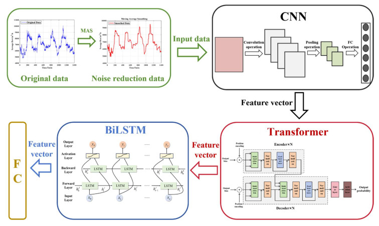
Accurate prediction of sewage flow is crucial for optimizing sewage treatment processes, cutting down energy consumption, and reducing pollution incidents. Current prediction models, including traditional statistical models and machine learning models, have limited performance when handling nonlinear and high-noise data. Although deep learning models excel in time series prediction, they still face challenges such as computational complexity, overfitting, and poor performance in practical applications. Accordingly, this study proposed a combined prediction model based on an improved sparrow search algorithm (SSA), convolutional neural network (CNN), transformer, and bidirectional long short-term memory network (BiLSTM) for sewage flow prediction. Specifically, the CNN part was responsible for extracting local features from the time series, the Transformer part captured global dependencies using the attention mechanism, and the BiLSTM part performed deep temporal processing of the features. The improved SSA algorithm optimized the model's hyperparameters to improve prediction accuracy and generalization capability. The proposed model was validated on a sewage flow dataset from an actual sewage treatment plant. Experimental results showed that the introduced Transformer mechanism significantly enhanced the ability to handle long time series data, and an improved SSA algorithm effectively optimized the hyperparameter selection, improving the model's prediction accuracy and training efficiency. After introducing an improved SSA, CNN, and Transformer modules, the prediction model's $ {R^{\text{2}}} $ increased by 0.18744, $ RMSE $ (root mean square error) decreased by 114.93, and $ MAE $ (mean absolute error) decreased by 86.67. The difference between the predicted peak/trough flow and monitored peak/trough flow was within 3.6% and the predicted peak/trough flow appearance time was within 2.5 minutes away from the monitored peak/trough flow time. By employing a multi-model fusion approach, this study achieved efficient and accurate sewage flow prediction, highlighting the potential and application prospects of the model in the field of sewage treatment.

| [1] |
W. Chen, J. Lim, S. Miyata, Y. Akashi, Exploring the spatial distribution for efficient sewage heat utilization in urban areas using the urban sewage state prediction model, Appl. Energ., 360 (2024), 122776. https://doi.org/10.1016/J.APENERGY.2024.122776 doi: 10.1016/J.APENERGY.2024.122776

|
| [2] |
Z. Jaffari, S. Na, A. Abbas, K. Y. Park, K. H. Cho, Digital imaging-in-flow (FlowCAM) and probabilistic machine learning to assess the sonolytic disinfection of cyanobacteria in sewage wastewater, J. Hazard. Mater., 468 (2024), 133762. https://doi.org/10.1016/J.JHAZMAT.2024.133762 doi: 10.1016/J.JHAZMAT.2024.133762
|
| [3] |
A. Osmane, K. Zidan, R. Benaddi, S. Sbahi, N. Ouazzani, M. Belmouden, et al., Assessment of the effectiveness of a full-scale trickling filter for the treatment of municipal sewage in an arid environment: Multiple linear regression model prediction of fecal coliform removal, J. Water Process Eng., 64 (2024), 105684. https://doi.org/10.1016/j.jwpe.2024.105684 doi: 10.1016/j.jwpe.2024.105684
|
| [4] |
M. Ansari, F. Othman, A. El-Shafie, Optimized fuzzy inference system to enhance prediction accuracy for influent characteristics of a sewage treatment plant, Sci. Total Environ., 722 (2020), 137878. https://doi.org/10.1016/j.scitotenv.2020.137878 doi: 10.1016/j.scitotenv.2020.137878
|
| [5] |
X. Wang, B. Zhao, X. Yang, Co-pyrolysis of microalgae and sewage sludge: Biocrude assessment and char yield prediction, Energy Convers. Manage., 117 (2016), 326–334. https://doi.org/10.1016/j.enconman.2016.03.013 doi: 10.1016/j.enconman.2016.03.013
|
| [6] |
V. Nourani, R. Zonouz, M. Dini, Estimation of prediction intervals for uncertainty assessment of artificial neural network based wastewater treatment plant effluent modeling, J. Water Process Eng., 55 (2023), 104145. https://doi.org/10.1016/j.jwpe.2023.104145 doi: 10.1016/j.jwpe.2023.104145
|
| [7] |
H. Mahanna, N. EL-Rahsidy, M. Kaloop, S. El-Sapakh, A. Alluqmani, R. Hassan, Prediction of wastewater treatment plant performance through machine learning techniques, Desalin. Water Treat., 14 (2024), 100524. https://doi.org/10.1016/j.dwt.2024.100524 doi: 10.1016/j.dwt.2024.100524
|
| [8] |
J. Li, K. Sharma, Y. Liu, G. Jiang, Z. Yuan, Real-time prediction of rain-impacted sewage flow for on-line control of chemical dosing in sewers, Water Res., 149 (2019), 311–321. https://doi.org/10.1016/j.watres.2018.11.021 doi: 10.1016/j.watres.2018.11.021
|
| [9] |
Y. Liu, X. Wu, W. Qi, Assessing the water quality in urban river considering the influence of rainstorm flood: A case study of Handan city, China, Ecol. Indic., 160 (2024), 111941. https://doi.org/10.1016/j.ecolind.2024.111941 doi: 10.1016/j.ecolind.2024.111941
|
| [10] |
E. Ekinci, B. Özbay, S. Omurca, F. Sayın, İ. Özbay, Application of machine learning algorithms and feature selection methods for better prediction of sludge production in a real advanced biological wastewater treatment plant, J. Environ. Manag., 348 (2023), 119448. https://doi.org/10.1016/j.jenvman.2023.119448 doi: 10.1016/j.jenvman.2023.119448
|
| [11] |
Z. Gao, J. Chen, G. Wang, S. Ren, L. Fang, Y. Aa, et al., A novel multivariate time series prediction of crucial water quality parameters with Long Short-Term Memory (LSTM) networks, J. Contam. Hydrol., 259 (2023), 104262. https://doi.org/10.1016/j.jconhyd.2023.104262 doi: 10.1016/j.jconhyd.2023.104262
|
| [12] |
M. Yaqub, H. Asif, S. Kim, W. Lee, Modeling of a full-scale sewage treatment plant to predict the nutrient removal efficiency using a long short-term memory (LSTM) neural network, J. Water Process Eng., 37 (2020), 101388. https://doi.org/10.1016/j.jwpe.2020.101388 doi: 10.1016/j.jwpe.2020.101388
|
| [13] |
N. Farhi, E. Kohen, H. Mamane, Y. Shavitt, Prediction of wastewater treatment quality using LSTM neural network, Environ. Technol. Inno., 23 (2021), 101632. https://doi.org/10.1016/j.eti.2021.101632 doi: 10.1016/j.eti.2021.101632
|
| [14] |
W. Alfwzan, M. Selim, A. Almalki, I. S. Alharbi, Water quality assessment using Bi-LSTM and computational fluid dynamics (CFD) techniques, Alex. Eng. J., 97 (2024), 346–359. https://doi.org/10.1016/j.aej.2024.04.030 doi: 10.1016/j.aej.2024.04.030
|
| [15] |
W. Zhang, J. Zhao, P. Quan, J. Wang, X. Meng, Q. Li, Prediction of influent wastewater quality based on wavelet transform and residual LSTM, Appl. Soft Comput., 148 (2023), 110858. https://doi.org/10.1016/j.asoc.2023.110858 doi: 10.1016/j.asoc.2023.110858
|
| [16] |
Y. Zhang, C. Li, Y. Jiang, L. Sun, R. Zhao, K. Yan, et al., Accurate prediction of water quality in urban drainage network with integrated EMD-LSTM model, J. Clean. Prod., 354 (2022), 131724. https://doi.org/10.1016/j.jclepro.2022.131724 doi: 10.1016/j.jclepro.2022.131724
|
| [17] |
L. Zheng, H. Wang, C. Liu, S. Zhang, A. Ding, E. Xie, et al., Prediction of harmful algal blooms in large water bodies using the combined EFDC and LSTM models, J. Environ. Manag., 295 (2021), 113060. https://doi.org/10.1016/j.jenvman.2021.113060 doi: 10.1016/j.jenvman.2021.113060
|
| [18] |
L. Zhang, C. Wang, W. Hu, X. Wang, H. Wang, X. Sun, et al., Dynamic real-time forecasting technique for reclaimed water volumes in urban river environmental management, Environ. Res., 248 (2024), 118267. https://doi.org/10.1016/j.envres.2024.118267 doi: 10.1016/j.envres.2024.118267
|
| [19] |
S. Huan, A novel interval decomposition correlation particle swarm optimization-extreme learning machine model for short-term and long-term water quality prediction, J. Hydrol., 625 (2023), 130034. https://doi.org/10.1016/j.jhydrol.2023.130034 doi: 10.1016/j.jhydrol.2023.130034
|
| [20] |
H. Darabi, A. Haghighi, O. Rahmati, A. Shahrood, S. Rouzbeh, B. Pradhan, et al., A hybridized model based on neural network and swarm intelligence-grey wolf algorithm for spatial prediction of urban flood-inundation, J. Hydrol., 603 (2021), 126854. https://doi.org/10.1016/j.jhydrol.2021.126854 doi: 10.1016/j.jhydrol.2021.126854
|
| [21] |
Z. Wang, H. Dai, B. Chen, S. Cheng, Y. Sun, J. Zhao, et al., Effluent quality prediction of the sewage treatment based on a hybrid neural network model: Comparison and application, J. Environ. Manag., 351 (2024), 119900. https://doi.org/10.1016/j.jenvman.2023.119900 doi: 10.1016/j.jenvman.2023.119900
|
| [22] |
F. Farzin, S. Moghaddam, M. Ehteshami, Auto-tuning data-driven model for biogas yield prediction from anaerobic digestion of sewage sludge at the south-tehran wastewater treatment plant: Feature selection and hyperparameter population-based optimization, Renew. Energy, 227 (2024), 120554. https://doi.org/10.1016/j.renene.2024.120554 doi: 10.1016/j.renene.2024.120554
|
| [23] |
G. Ye, J. Wan, Z. Deng, Y. Wang, J. Chen, B. Zhu, et al., Prediction of effluent total nitrogen and energy consumption in wastewater treatment plants: Bayesian optimization machine learning methods, Bioresource Technol., 395 (2024), 130361. https://doi.org/10.1016/j.biortech.2024.130361 doi: 10.1016/j.biortech.2024.130361
|
| [24] |
J. Piri, B. Pirzadeh, B. Keshtegar, M. Givehchi, Reliability analysis of pumping station for sewage network using hybrid neural networks-genetic algorithm and method of moment, Process Saf. Environ., 145 (2021), 39–51. https://doi.org/10.1016/j.psep.2020.07.045 doi: 10.1016/j.psep.2020.07.045
|
| [25] |
M. Salamattalab, M. Zonoozi, M. Molavi-Arabshahi, Innovative approach for predicting biogas production from large-scale anaerobic digester using long-short term memory (LSTM) coupled with genetic algorithm (GA), Waste Manag., 175 (2024), 30–41. https://doi.org/10.1016/j.wasman.2023.12.046 doi: 10.1016/j.wasman.2023.12.046
|
| [26] |
A. Mohammed, K. Hassan, M. Abdel-Aal, Moving average smoothing for gregory-newton interpolation: A novel approach for short-term demand forecasting, IFAC-PapersOnLine, 55 (2022), 749–754. https://doi.org/10.1016/j.ifacol.2022.09.499 doi: 10.1016/j.ifacol.2022.09.499
|
| [27] |
P. Mei, M. Li, Q. Zhang, G. Li, L. Song, Prediction model of drinking water source quality with potential industrial-agricultural pollution based on CNN-GRU-Attention, J. Hydrol., 610 (2022), 127934. https://doi.org/10.1016/j.jhydrol.2022.127934 doi: 10.1016/j.jhydrol.2022.127934
|
| [28] |
A. L. de Rojas, M. A. Jaramillo-Morán, J. E. Sandubete, EMDFormer model for time series forecasting, AIMS Math., 9 (2024), 9419–9434. https://doi.org/10.3934/math.2024459 doi: 10.3934/math.2024459
|
| [29] |
H. Jin, Y. Liang, H. Lu, S. Zhang, Y. Gao, Y. Zhao, et al., An intelligent framework for spatiotemporal simulation of flooding considering urban underlying surface characteristics, Int. J. Appl. Earth Obs., 130 (2024), 103908. https://doi.org/10.1016/j.jag.2024.103908 doi: 10.1016/j.jag.2024.103908
|
| [30] |
B. Qu, E. Jiang, J. Li, Y. Liu, C. Liu, Coupling coordination relationship of water resources, eco-environment and socio-economy in the water-receiving area of the Lower Yellow River, Ecol. Indic., 160 (2024), 111766. https://doi.org/10.1016/j.ecolind.2024.111766 doi: 10.1016/j.ecolind.2024.111766
|
| [31] |
J. Cai, B. Sun, H. Wang, Y. Zheng, S. Zhou, H. Li, et al., Application of the improved dung beetle optimizer, muti-head attention and hybrid deep learning algorithms to groundwater depth prediction in the Ningxia area, China, Atmos. Ocean. Sci. Lett., 2024, 100497. https://doi.org/10.1016/j.aosl.2024.100497 doi: 10.1016/j.aosl.2024.100497
|
| [32] |
M. Wang, G. Zhao, S. Wang, Hybrid random forest models optimized by Sparrow search algorithm (SSA) and Harris hawk optimization algorithm (HHO) for slope stability prediction, Transp. Geotech., 48 (2024), 101305. https://doi.org/10.1016/j.trgeo.2024.101305 doi: 10.1016/j.trgeo.2024.101305
|
| [33] |
C. Zhang, S. Ding, A stochastic configuration network based on chaotic sparrow search algorithm, Knowl.-Based Syst., 220 (2024), 106924. https://doi.org/10.1016/j.knosys.2021.106924 doi: 10.1016/j.knosys.2021.106924
|
| [34] |
X. Shao, J. Yu, Z. Li, X. Yang, B. Sundén, Energy-saving optimization of the parallel chillers system based on a multi-strategy improved sparrow search algorithm, Heliyon, 9 (2023), e21012. https://doi.org/10.1016/j.heliyon.2023.e21012 doi: 10.1016/j.heliyon.2023.e21012
|
| [35] |
X. Long, W. Cai, L. Yang, H. Huang, Improved particle swarm optimization with reverse learning and neighbor adjustment for space surveillance network task scheduling, Swarm Evol. Comput., 85 (2024), 101482. https://doi.org/10.1016/j.swevo.2024.101482 doi: 10.1016/j.swevo.2024.101482
|
| [36] |
S. Zhao, Y. Duan, N. Roy, B. Zhang, A deep learning methodology based on adaptive multiscale CNN and enhanced highway LSTM for industrial process fault diagnosis, Reliab. Eng. Syst. Safe., 249 (2024), 110208. https://doi.org/10.1016/j.ress.2024.110208 doi: 10.1016/j.ress.2024.110208
|
| [37] |
K. Wang, X. Fan, X. Yang, Z. Zhou, An AQI decomposition ensemble model based on SSA-LSTM using improved AMSSA-VMD decomposition reconstruction technique, Environ. Res., 232 (2023), 116365. https://doi.org/10.1016/j.envres.2023.116365 doi: 10.1016/j.envres.2023.116365
|
| [38] |
Y. Leng, H. Zhang, X. Li, A novel evaluation method for renewable energy development based on improved sparrow search algorithm and projection pursuit model, Expert Syst. Appl., 244 (2024), 122991. https://doi.org/10.1016/j.eswa.2023.122991 doi: 10.1016/j.eswa.2023.122991
|
| [39] |
Z. Zhang, X. Cheng, Z. Xing, Z. Wang, Y. Qin, Optimal sizing of battery-supercapacitor energy storage systems for trams using improved PSO algorithm, J. Energy Storage, 73 (2023), 108962. https://doi.org/10.1016/j.est.2023.108962 doi: 10.1016/j.est.2023.108962
|
| [40] |
J. Li, R. Liu, R. Wang, Handling dynamic capacitated vehicle routing problems based on adaptive genetic algorithm with elastic strategy, Swarm Evol. Comput., 86 (2024), 101529. https://doi.org/10.1016/j.swevo.2024.101529 doi: 10.1016/j.swevo.2024.101529
|
| [41] |
X. Zhang, J. Xia, Z. Chen, J. Zhu, H. Wang, A nutrient optimization method for hydroponic lettuce based on multi-strategy improved grey wolf optimizer algorithm, Comput. Electron. Agr., 224 (2024), 109167. https://doi.org/10.1016/j.compag.2024.109167 doi: 10.1016/j.compag.2024.109167
|
| [42] |
J. Sahayaraj, K. Gunasekaran, S. Verma, M. Dhurgadevi, Energy efficient clustering and sink mobility protocol using improved dingo and boosted beluga whale optimization algorithm for extending network lifetime in WSNs, Sustain. Comput.-Infor., 43 (2024), 101008. https://doi.org/10.1016/j.suscom.2024.101008 doi: 10.1016/j.suscom.2024.101008
|
| [43] |
F. Zhu, G. Li, H. Tang, Y. Li, X. Lv, X.Wang, Dung beetle optimization algorithm based on quantum computing and multi-strategy fusion for solving engineering problems, Expert Syst. Appl., 236 (2024), 121219. https://doi.org/10.1016/j.eswa.2023.121219 doi: 10.1016/j.eswa.2023.121219
|
| [44] |
L. Yin, W. Ding, Deep neural network accelerated-group african vulture optimization algorithm for unit commitment considering uncertain wind power, Appl. Soft Comput., 162 (2024), 111845. https://doi.org/10.1016/j.asoc.2024.111845 doi: 10.1016/j.asoc.2024.111845
|
| [45] |
M. Abdel-Basset, R. Mohamed, M. Abouhawwash, Crested porcupine optimizer: A new nature-inspired metaheuristic, Knowl.-Based Syst., 284 (2024), 111257. https://doi.org/10.1016/j.knosys.2023.111257 doi: 10.1016/j.knosys.2023.111257
|
| [46] |
U. Khan, N. Khan, M. Zafar, Resource efficient PV power forecasting: Transductive transfer learning based hybrid deep learning model for smart grid in Industry 5.0, Energy Convers. Man.-X, 20 (2024), 100486. https://doi.org/10.1016/j.ecmx.2023.100486 doi: 10.1016/j.ecmx.2023.100486
|
| [47] |
X. Zhou, B. Sheil, S. Suryasentana, P. Shi, Multi-fidelity fusion for soil classification via LSTM and multi-head self-attention CNN model, Adv. Eng. Inform., 62 (2024), 102655. https://doi.org/10.1016/j.aei.2024.102655 doi: 10.1016/j.aei.2024.102655
|
| [48] |
M. Javanmard, S. Ghaderi, A hybrid model with applying machine learning algorithms and optimization model to forecast greenhouse gas emissions with energy market data, Sustain. Cities Soc., 82 (2022), 103886. https://doi.org/10.1016/j.scs.2022.103886 doi: 10.1016/j.scs.2022.103886
|
| [49] |
S. Tariq, J. Loy-Benitez, K. Nam, S. Kim, M. Kim, C. Yoo, Deep-AI soft sensor for sustainable health risk monitoring and control of fine particulate matter at sesnsor devoid underground spaces: A zero-shot transfer learning approach, Tunn. Undergr. Sp. Tech., 131 (2023), 104843. https://doi.org/10.1016/j.tust.2022.104843 doi: 10.1016/j.tust.2022.104843
|
| [50] |
Z. Wang, N. Xu, X. Bao, J. Wu, X. Cui, Spatio-temporal deep learning model for accurate streamflow prediction with multi-source data fusion, Environ. Modell. Softw., 178 (2024), 106091. https://doi.org/10.1016/j.envsoft.2024.106091 doi: 10.1016/j.envsoft.2024.106091
|
| [51] |
G. Dai, Z. Tian, J. Fan, C. K. Sunil, C. Dewi, DFN-PSAN: Multi-level deep information feature fusion extraction network for interpretable plant disease classification, Comput. Electron. Agr., 216 (2024), 108481. https://doi.org/10.1016/j.compag.2023.108481 doi: 10.1016/j.compag.2023.108481
|


Figures(21) / Tables(10)

Jiawen Ye, Lei Dai, Haiying Wang. Enhancing sewage flow prediction using an integrated improved SSA-CNN-Transformer-BiLSTM model[J]. AIMS Mathematics, 2024, 9(10): 26916-26950. doi: 10.3934/math.20241310


 DownLoad: