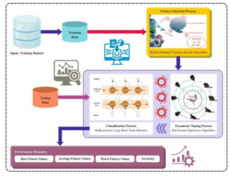
The latest advances in engineering, science, and technology have contributed to an enormous generation of datasets. This vast dataset contains irrelevant, redundant, and noisy features that adversely impact classification performance in data mining and machine learning (ML) techniques. Feature selection (FS) is a preprocessing stage to minimize the data dimensionality by choosing the most prominent feature while improving the classification performance. Since the size data produced are often extensive in dimension, this enhances the complexity of search space, where the maximal number of potential solutions is 2nd for n feature datasets. As n becomes large, it becomes computationally impossible to compute the feature. Therefore, there is a need for effective FS techniques for large-scale problems of classification. Many metaheuristic approaches were utilized for FS to resolve the challenges of heuristic-based approaches. Recently, the swarm algorithm has been suggested and demonstrated to perform effectively for FS tasks. Therefore, I developed a Hybrid Mutated Tunicate Swarm Algorithm for FS and Global Optimization (HMTSA-FSGO) technique. The proposed HMTSA-FSGO model mainly aims to eradicate unwanted features and choose the relevant ones that highly impact the classifier results. In the HMTSA-FSGO model, the HMTSA is derived by integrating the standard TSA with two concepts: A dynamic s-best mutation operator for an optimal trade-off between exploration and exploitation and a directional mutation rule for enhanced search space exploration. The HMTSA-FSGO model also includes a bidirectional long short-term memory (BiLSTM) classifier to examine the impact of the FS process. The rat swarm optimizer (RSO) model can choose the hyperparameters to boost the BiLSTM network performance. The simulation analysis of the HMTSA-FSGO technique is tested using a series of experiments. The investigational validation of the HMTSA-FSGO technique showed a superior outcome of 93.01%, 97.39%, 61.59%, 99.15%, and 67.81% over diverse datasets.
Citation: Turki Althaqafi. Mathematical modeling of a Hybrid Mutated Tunicate Swarm Algorithm for Feature Selection and Global Optimization[J]. AIMS Mathematics, 2024, 9(9): 24336-24358. doi: 10.3934/math.20241184
The latest advances in engineering, science, and technology have contributed to an enormous generation of datasets. This vast dataset contains irrelevant, redundant, and noisy features that adversely impact classification performance in data mining and machine learning (ML) techniques. Feature selection (FS) is a preprocessing stage to minimize the data dimensionality by choosing the most prominent feature while improving the classification performance. Since the size data produced are often extensive in dimension, this enhances the complexity of search space, where the maximal number of potential solutions is 2nd for n feature datasets. As n becomes large, it becomes computationally impossible to compute the feature. Therefore, there is a need for effective FS techniques for large-scale problems of classification. Many metaheuristic approaches were utilized for FS to resolve the challenges of heuristic-based approaches. Recently, the swarm algorithm has been suggested and demonstrated to perform effectively for FS tasks. Therefore, I developed a Hybrid Mutated Tunicate Swarm Algorithm for FS and Global Optimization (HMTSA-FSGO) technique. The proposed HMTSA-FSGO model mainly aims to eradicate unwanted features and choose the relevant ones that highly impact the classifier results. In the HMTSA-FSGO model, the HMTSA is derived by integrating the standard TSA with two concepts: A dynamic s-best mutation operator for an optimal trade-off between exploration and exploitation and a directional mutation rule for enhanced search space exploration. The HMTSA-FSGO model also includes a bidirectional long short-term memory (BiLSTM) classifier to examine the impact of the FS process. The rat swarm optimizer (RSO) model can choose the hyperparameters to boost the BiLSTM network performance. The simulation analysis of the HMTSA-FSGO technique is tested using a series of experiments. The investigational validation of the HMTSA-FSGO technique showed a superior outcome of 93.01%, 97.39%, 61.59%, 99.15%, and 67.81% over diverse datasets.

| [1] | M. Sharawi, H. M. Zawbaa, E. Emary, H. M. Zawbaa, E. Emary, Feature selection approach based on whale optimization algorithm, in 2017 Ninth International Conference on Advanced Computational Intelligence (ICACI), 163–168. https://doi.org/10.1109/ICACI.2017.7974502 |
| [2] |
G. I. Sayed, A. Darwish, A. E. Hassanien, A new chaotic whale optimization algorithm for features selection, J. Classification, 35 (2018), 300–344. https://doi.org/10.1007/s00357-018-9261-2 doi: 10.1007/s00357-018-9261-2

|
| [3] |
K. Chen, F. Y. Zhou, X. F. Yuan, Hybrid particle swarm optimization with spiral-shaped mechanism for feature selection, Expert Syst. Appl., 128 (2019), 140–156. https://doi.org/10.1016/j.eswa.2019.03.039 doi: 10.1016/j.eswa.2019.03.039
|
| [4] |
M. Ragab, Hybrid firefly particle swarm optimisation algorithm for feature selection problems, Expert Syst., 41 (2024), e13363. https://doi.org/10.1111/exsy.13363 doi: 10.1111/exsy.13363
|
| [5] |
H. Faris, M. A. Hassonah, A. M. Al-Zoubi, S. Mirjalili, I. Aljarah, A multi-verse optimizer approach for feature selection and optimizing SVM parameters based on a robust system architecture, Neural Comput. Appl., 30 (2018), 2355–2369. https://doi.org/10.1007/s00521-016-2818-2 doi: 10.1007/s00521-016-2818-2
|
| [6] |
S. Gu, R. Cheng, Y. Jin, Feature selection for high-dimensional classification using a competitive swarm optimizer, Soft Comput., 22 (2018), 811–822. https://doi.org/10.1007/s00521-016-2818-2 doi: 10.1007/s00521-016-2818-2
|
| [7] |
Q. Tu, X. Chen, X. Liu, Hierarchy strengthened grey wolf optimizer for numerical optimization and feature selection, IEEE Access, 7 (2019), 78012–78028. https://doi.org/10.1109/ACCESS.2019.2921793 doi: 10.1109/ACCESS.2019.2921793
|
| [8] |
F. Hafiz, A. Swain, N. Patel, C. Naik, A two-dimensional (2-D) learning framework for particle swarm based feature selection, Pattern Recognit., 76 (2018), 416–433. https://doi.org/10.1016/j.patcog.2017.11.027 doi: 10.1016/j.patcog.2017.11.027
|
| [9] |
M. Ragab, Multi-Label scene classification on remote sensing imagery using modified Dingo Optimizer with deep learning, IEEE Access, 12 (2024), 11879–11886. https://doi.org/10.1109/ACCESS.2023.3344773 doi: 10.1109/ACCESS.2023.3344773
|
| [10] | R. C. T. De Souza, L. D. S. Coelho, C. A. De Macedo, J. Pierezan, A V-Shaped binary crow search algorithm for feature selection, in 2018 IEEE Congress on Evolutionary Computation (CEC), 2018, 1–8. https://doi.org/10.1109/CEC.2018.8477975 |
| [11] |
E. H. Houssein, A. Hammad, M. M. Emam, A. A. Ali, An enhanced Coati Optimization Algorithm for global optimization and feature selection in EEG emotion recognition, Comput. Biol. Med., 173 (2024), 108329. https://doi.org/10.1016/j.compbiomed.2024.108329 doi: 10.1016/j.compbiomed.2024.108329
|
| [12] |
M. Chaibi, L. Tarik, M. Berrada, A. El Hmaidi, Machine learning models based on random forest feature selection and Bayesian optimization for predicting daily global solar radiation, Inter. J. Renew. Energy D., 11 (2022), 309. https://doi.org/10.14710/ijred.2022.41451 doi: 10.14710/ijred.2022.41451
|
| [13] |
R. R. Mostafa, M. A. Gaheen, M. Abd ElAziz, M. A. Al-Betar, A. A. Ewees, An improved gorilla troops optimizer for global optimization problems and feature selection, Knowl.-Based Syst., 269 (2023), 110462. https://doi.org/10.1016/j.knosys.2023.110462 doi: 10.1016/j.knosys.2023.110462
|
| [14] |
B. D. Kwakye, Y. Li, H. H. Mohamed, E. Baidoo, T. Q. Asenso, Particle guided metaheuristic algorithm for global optimization and feature selection problems, Expert Syst. Appl., 248 (2024), 123362. https://doi.org/10.1016/j.eswa.2024.123362 doi: 10.1016/j.eswa.2024.123362
|
| [15] |
E. H. Houssein, M. E. Hosney, D. Oliva, E. M. Younis, A. A. Ali, W. M. Mohamed, An efficient discrete rat swarm optimizer for global optimization and feature selection in chemoinformatics, Knowl.-Based Syst., 275 (2023), 110697. https://doi.org/10.1016/j.knosys.2023.110697 doi: 10.1016/j.knosys.2023.110697
|
| [16] |
M. Qaraad, S. Amjad, N. K. Hussein, M. A. Elhosseini, 2022. Large scale salp-based grey wolf optimization for feature selection and global optimization, Neural Comput. Appl., 34 (11), 8989–9014. https://doi.org/10.1007/s00521-022-06921-2 doi: 10.1007/s00521-022-06921-2
|
| [17] |
L. Abualigah, M. Altalhi, A novel generalized normal distribution arithmetic optimization algorithm for global optimization and data clustering problems, J. Amb. Intel. Hum. Comput., 15 (2024), 389–417. https://doi.org/10.1007/s12652-022-03898-7 doi: 10.1007/s12652-022-03898-7
|
| [18] |
B. Xu, A. A. Heidari, Z. Cai, H. Chen, Dimensional decision covariance colony predation algorithm: global optimization and high− dimensional feature selection, Artif. Intell. Rev., 56 (2023), 11415–11471. https://doi.org/10.1007/s10462-023-10412-8 doi: 10.1007/s10462-023-10412-8
|
| [19] |
T. Si, P. B. Miranda, U. Nandi, N. D. Jana, S. Mallik, U. Maulik, Opposition-based Chaotic Tunicate Swarm Algorithms for Global Optimization, IEEE Access, 12 (2024), 18168–18188. https://doi.org/10.1109/ACCESS.2024.3359587 doi: 10.1109/ACCESS.2024.3359587
|
| [20] |
G. Liu, Z. Guo, W. Liu, B. Cao, S. Chai, C.Wang, MSHHOTSA: A variant of tunicate swarm algorithm combining multi-strategy mechanism and hybrid Harris optimization, Plos one, 18 (2023), e0290117. https://doi.org/10.1371/journal.pone.0290117 doi: 10.1371/journal.pone.0290117
|
| [21] |
A. Alizadeh, F. S. Gharehchopogh, M. Masdari, A. Jafarian, An improved hybrid salp swarm optimization and African vulture optimization algorithm for global optimization problems and its applications in stock market prediction, Soft Comput., 28 (2024), 5225–5261. https://doi.org/10.1007/s00500-023-09299-y doi: 10.1007/s00500-023-09299-y
|
| [22] |
Z. Pan, D. Lei, L. Wang, A knowledge-based two-population optimization algorithm for distributed energy-efficient parallel machines scheduling, IEEE T. Cybernetics, 52 (2020), 5051–5063. https://doi.org/10.1109/TCYB.2020.3026571 doi: 10.1109/TCYB.2020.3026571
|
| [23] |
F. Zhao, S. Di, L. Wang, A hyperheuristic with Q-learning for the multiobjective energy-efficient distributed blocking flow shop scheduling problem, IEEE T. Cybernetics, 53 (2022), 3337–3350. https://doi.org/10.1109/TCYB.2022.3192112 doi: 10.1109/TCYB.2022.3192112
|
| [24] |
F. Zhao, C. Zhuang, L. Wang, C. Dong, An Iterative Greedy Algorithm With $ Q $-Learning Mechanism for the Multiobjective Distributed No-Idle Permutation Flowshop Scheduling, IEEE Transactions on Systems, Man, and Cybernetics: Systems, 2024. https://doi.org/10.1109/TSMC.2024.3358383 doi: 10.1109/TSMC.2024.3358383
|
| [25] |
V. Chandran, P. Mohapatra, A Novel Multi-Strategy Ameliorated Quasi-Oppositional Chaotic Tunicate Swarm Algorithm for Global Optimization and Constrained Engineering Applications, Heliyon, 2024. https://doi.org/10.1016/j.heliyon.2024.e30757 doi: 10.1016/j.heliyon.2024.e30757
|
| [26] |
F. A. Hashim, E. H. Houssein, R. R. Mostafa, A. G. Hussien, F. Helmy, An efficient adaptive-mutated Coati optimization algorithm for feature selection and global optimization, Alexandria Eng. J., 85 (2023), 29–48. https://doi.org/10.1016/j.aej.2023.11.004 doi: 10.1016/j.aej.2023.11.004
|
| [27] |
A. S. AL-Ghamdi, M. Ragab, Tunicate swarm algorithm with deep convolutional neural network-driven colorectal cancer classification from histopathological imaging data, Electron. Res. Arch., 31 (2023), 2793–2812. https://doi.org/10.3934/era.2023141 doi: 10.3934/era.2023141
|
| [28] |
A. Adamu, M. Abdullahi, S. B. Junaidu, I. H. Hassan, An hybrid particle swarm optimization with crow search algorithm for feature selection, Machine Learn. Appl., 6 (2021), 100108. https://doi.org/10.1016/j.mlwa.2021.100108 doi: 10.1016/j.mlwa.2021.100108
|
| [29] |
A. Kumar, S. R. Sangwan, A. Arora, A. Nayyar, M. Abdel-Basset, Sarcasm detection using soft attention-based bidirectional long short-term memory model with convolution network, IEEE Access, 7 (2019), 23319–23328. https://doi.org/10.1109/ACCESS.2019.2899260 doi: 10.1109/ACCESS.2019.2899260
|
| [30] | I. M. Batiha, B. Mohamed, Binary rat swarm optimizer algorithm for computing independent domination metric dimension problem, 2024. https://doi.org/10.1109/ACCESS.2019.2899260 |
| [31] | https://archive.ics.uci.edu/datasets |
| [32] |
A. E. Hegazy, M. A. Makhlouf, G. S. El-Tawel, Improved salp swarm algorithm for feature selection, J. King Saud Univ-Com, 32 (2020), 335–344. https://doi.org/10.1109/ACCESS.2019.2899260 doi: 10.1109/ACCESS.2019.2899260
|


Figures(10) / Tables(7)

Turki Althaqafi. Mathematical modeling of a Hybrid Mutated Tunicate Swarm Algorithm for Feature Selection and Global Optimization[J]. AIMS Mathematics, 2024, 9(9): 24336-24358. doi: 10.3934/math.20241184


 DownLoad: