In the last few decades, the particle swarm optimization (PSO) algorithm has been demonstrated to be an effective approach for solving real-world optimization problems. To improve the effectiveness of the PSO algorithm in finding the global best solution for constrained optimization problems, we proposed an improved composite particle swarm optimization algorithm (ICPSO). Based on the optimization principles of the PSO algorithm, in the ICPSO algorithm, we constructed an evolutionary update mechanism for the personal best position population. This mechanism incorporated composite concepts, specifically the integration of the $ \varepsilon $-constraint, differential evolution (DE) strategy, and feasibility rule. This approach could effectively balance the objective function and constraints, and could improve the ability of local exploitation and global exploration. Experiments on the CEC2006 and CEC2017 benchmark functions and real-world constraint optimization problems from the CEC2020 dataset showed that the ICPSO algorithm could effectively solve complex constrained optimization problems.
Citation: Ying Sun, Yuelin Gao. An improved composite particle swarm optimization algorithm for solving constrained optimization problems and its engineering applications[J]. AIMS Mathematics, 2024, 9(4): 7917-7944. doi: 10.3934/math.2024385
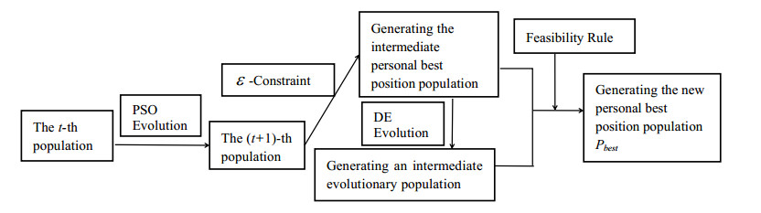
In the last few decades, the particle swarm optimization (PSO) algorithm has been demonstrated to be an effective approach for solving real-world optimization problems. To improve the effectiveness of the PSO algorithm in finding the global best solution for constrained optimization problems, we proposed an improved composite particle swarm optimization algorithm (ICPSO). Based on the optimization principles of the PSO algorithm, in the ICPSO algorithm, we constructed an evolutionary update mechanism for the personal best position population. This mechanism incorporated composite concepts, specifically the integration of the $ \varepsilon $-constraint, differential evolution (DE) strategy, and feasibility rule. This approach could effectively balance the objective function and constraints, and could improve the ability of local exploitation and global exploration. Experiments on the CEC2006 and CEC2017 benchmark functions and real-world constraint optimization problems from the CEC2020 dataset showed that the ICPSO algorithm could effectively solve complex constrained optimization problems.

| [1] |
W. W. Jia, T. W. Huang, S. T. Qin, A collective neurodynamic penalty approach to nonconvex distributed constrained optimization, Neural Netw., 171 (2024), 145–158. https://doi.org/10.1016/j.neunet.2023.12.011 doi: 10.1016/j.neunet.2023.12.011

|
| [2] |
R. Y. Xu, J. Y. Tian, J. F. Li, X. P. Zhai, Trajectory planning of rail inspection robot based on an improved penalty function simulated annealing particle swarm algorithm, Int. J. Control Autom. Syst., 21 (2023), 3368–3381. https://doi.org/10.1007/s12555-022-0163-z doi: 10.1007/s12555-022-0163-z
|
| [3] |
Y. Wang, B. C. Wang, H. X. Li, G. G. Yen, Incorporating objective function information into the feasibility rule for constrained evolutionary optimization, IEEE Trans. Cybern., 46 (2016), 2938–2952. https://doi.org/10.1109/TCYB.2015.2493239 doi: 10.1109/TCYB.2015.2493239
|
| [4] |
W. C. Wang, W. C. Tian, K. Chau, H. F. Zang, M. W. Ma, Z. K. Feng, et al., Multi-reservoir flood control operation using improved bald eagle search algorithm with $\varepsilon$-constraint method, Water, 15 (2023), 1–24. https://doi.org/10.3390/w15040692 doi: 10.3390/w15040692
|
| [5] |
Y. Wang, Z. X. Cai, G. Q. Guo, Y. R. Zhou, Multiobjective optimization and hybrid evolutionary algorithm to solve constrained optimization problems, IEEE Trans. Syst. Man Cybern. B, 37 (2007), 560–575. https://doi.org/10.1109/tsmcb.2006.886164 doi: 10.1109/tsmcb.2006.886164
|
| [6] |
M. A. Jan, M. Sagheer, H. U. Khan, M. I. Uddin, R. A. Khanum, M. Mahmoud, et al., Hybrid stochastic ranking for constrained optimization, IEEE Access, 8 (2020), 227270–227287. https://doi.org/10.1109/ACCESS.2020.3044439 doi: 10.1109/ACCESS.2020.3044439
|
| [7] |
D. Karaboga, B. Akay, A modified artificial bee colony (ABC) algorithm for constrained optimization problems, Appl. Soft Comput., 11 (2011), 3021–3031. https://doi.org/10.1016/j.asoc.2010.12.001 doi: 10.1016/j.asoc.2010.12.001
|
| [8] |
J. P. Shi, P. S. Li, G. P. Liu, P. Liu, Improved fruit fly optimization algorithm for solving constrained problems and engineering applications (Chinese), Control Decis., 36 (2021), 314–324. https://doi.org/10.13195/j.kzyjc.2019.0557 doi: 10.13195/j.kzyjc.2019.0557
|
| [9] |
H. M. Jia, S. Z. Shi, D. Wu, H. H. Rao, J. R. Zhang, L. Abualigah, Improve coati optimization algorithm for solving constrained engineering optimization problems, J. Comput. Des. Eng., 10 (2023), 2223–2250. https://doi.org/10.1093/jcde/qwad095 doi: 10.1093/jcde/qwad095
|
| [10] |
B. C. Wang, H. X. Li, J. P. Li, Y. Wang, Composite differential evolution for constrained evolutionary optimization, IEEE Trans. Syst. Man Cybern. Syst., 49 (2019), 1482–1495. https://doi.org/10.1109/TSMC.2018.2807785 doi: 10.1109/TSMC.2018.2807785
|
| [11] |
F. L. Wang, G. Xu, M. Wang, An improved genetic algorithm for constrained optimization problems, IEEE Access, 11 (2023), 10032–10044. https://doi.org/10.1109/ACCESS.2023.3240467 doi: 10.1109/ACCESS.2023.3240467
|
| [12] |
H. Peng, Z. Z. Xu, J. Y. Qian, X. G. Dong, W. Li, Z. J. Wu, Evolutionary constrained optimization with hybrid constraint-handling technique, Expert Syst. Appl., 211 (2023), 118660. https://doi.org/10.1016/j.eswa.2022.118660 doi: 10.1016/j.eswa.2022.118660
|
| [13] | J. Kennedy, R. Eberhart, Particle swarm optimization, In: Proceedings of ICNN'95-International Conference on Neural Networks, 4 (1995), 1942–1948. https://doi.org/10.1109/ICNN.1995.488968 |
| [14] |
Karishma, H. Kumar, A new hybrid particle swarm optimizationalgorithm for optimal tasks scheduling in distributed computing system, Intell. Syst. Appl., 18 (2023), 200219. https://doi.org/10.1016/j.iswa.2023.200219 doi: 10.1016/j.iswa.2023.200219
|
| [15] |
H. C. Lu, H. Y. Tseng, S. W. Lin, Double-track particle swarm optimizer for nonlinear constrained optimization problems, Inform. Sci., 662 (2023), 587–628. https://doi.org/10.1016/j.ins.2022.11.164 doi: 10.1016/j.ins.2022.11.164
|
| [16] |
H. Liu, Z. X. Cai, Y. Wang, Hybridizing particle swarm optimization with differential evolution for constrained numerical and engineering optimization, Appl. Soft Comput., 10 (2010), 629–640. https://doi.org/10.1016/j.asoc.2009.08.031 doi: 10.1016/j.asoc.2009.08.031
|
| [17] |
Y. Wang, Z. X. Cai, A hybrid multi-swarm particle swarm optimization to solve constrained optimization problems, Front. Comput. Sci. China, 3 (2009), 38–52. https://doi.org/10.1007/s11704-009-0010-x doi: 10.1007/s11704-009-0010-x
|
| [18] |
E. Y. Guo, Y. L. Gao, C. Y. Hu, J. J. Zhang, A hybrid PSO-DE intelligent algorithm for solving constrained optimization problems based on feasibility rules, Mathematics, 11 (2023), 1–34. https://doi.org/10.3390/math11030522 doi: 10.3390/math11030522
|
| [19] |
G. Venter, R. T. Haftka, Constrained particle swarm optimization using a bi-objective formulation, Struct. Multidiscip. Optim., 40 (2010), 65–76. https://doi.org/10.1007/s00158-009-0380-6 doi: 10.1007/s00158-009-0380-6
|
| [20] |
K. M. Ang, W. H. Lim, N. A. M. Isa, S. S. Tiang, C. H. Wong, A constrained multi-swarm particle swarm optimization without velocity for constrained optimization problems, Expert Syst. Appl., 140 (2020), 112882. https://doi.org/10.1016/j.eswa.2019.112882 doi: 10.1016/j.eswa.2019.112882
|
| [21] | Y. Shi, R. Eberhart, A modified particle swarm optimizer, In: 1998 IEEE International Conference on Evolutionary Computation Proceedings, 1998, 69–73. https://doi.org/10.1109/ICEC.1998.699146 |
| [22] |
K. Deb, An efficient constraint handling method for genetic algorithms, Comput. Method. Appl. Mech. Eng., 186 (2000), 311–338. https://doi.org/10.1016/S0045-7825(99)00389-8 doi: 10.1016/S0045-7825(99)00389-8
|
| [23] | T. Takahama, S. Sakai, Constrained optimization by the $\varepsilon$ constrained differential evolution with an archive and gradient-based mutation, IEEE Congress on Evolutionary Computation, Spain: Barcelona, 2010, 1–9. https://doi.org/10.1109/CEC.2010.5586484 |
| [24] |
Z. Liu, Z. Y. Li, P. Zhu, W. Chen, A parallel boundary search particle swarm optimization algorithm for constrained optimization problems, Struct. Multidiscip. Optim., 58 (2018), 1505–1522. https://doi.org/10.1007/s00158-018-1978-3 doi: 10.1007/s00158-018-1978-3
|
| [25] | J. J. Liang, T. P. Runarsson, E. Mezura-Montes, M. Clerc, P. N. Suganthan, C. A. C. Coello, et al., Problem definitions and evaluation criteria for the CEC 2006 special session on constrained real-parameter optimization, Technical Report, Singapore: Nangyang Technological University, 2006, 1–24. |
| [26] | G. Wu, R. Mallipeddi, P. Suganthan, Problem definitions and evaluation criteria for the CEC 2017 competition and special session on constrained single objective real-parameter optimization, Technical Report, Singapore: Nangyang Technological University, 2017, 1–18. |
| [27] |
A. Kumar, G. H. Wu, M. Z. Ali, R. Mallipeddi, P. N. Suganthan, S. Das, A test-suite of non-convex constrained optimization problems from the real-world and some baseline results, Swarm Evol. Comput., 56 (2020), 100693. https://doi.org/10.1016/j.swevo.2020.100693 doi: 10.1016/j.swevo.2020.100693
|
| [28] | A. Kumar, S. Das, I. Zelinka, A self-adaptive spherical search algorithm for real-world constrained optimization problems, In: Proceedings of the 2020 Genetic and Evolutionary Computation Conference Companion, 2020, 13–14. https://doi.org/10.1145/3377929.3398186 |
| [29] |
J. Gurrola-Ramos, A. Hernàndez-Aguirre, O. Dalmau-Cedeño, COLSHADE for real-world single-objective constrained optimization problems, 2020 IEEE Congress on Evolutionary Computation (CEC), 2020, 1–8. https://doi.org/10.1109/CEC48606.2020.9185583 doi: 10.1109/CEC48606.2020.9185583
|
| [30] | A. Kumar, S. Das, I. Zelinka, A modified covariance matrix adaptation evolution strategy for real-world constrained optimization problems, In: Proceedings of the 2020 Genetic and Evolutionary Computation Conference Companion, 2020, 11–12. https://doi.org/10.1145/3377929.3398185 |
| [31] |
C. He, L. H. Li, Y. Tian, X. Y. Zhang, R. Cheng, Y. C. Jin, et al., Accelerating large-scale multiobjective optimization via problem reformulation, IEEE Trans. Evol. Comput., 23 (2019), 949–961. https://doi.org/10.1109/TEVC.2019.2896002 doi: 10.1109/TEVC.2019.2896002
|
| [32] | S. C. Liu, N. Lu, W. J. Hong, C. Qian, K. Tang, Effective and imperceptible adversarial textual attack via multi-objectivization, 2021, arXiv: 2111.01528. |


Figures(6) / Tables(10)

Ying Sun, Yuelin Gao. An improved composite particle swarm optimization algorithm for solving constrained optimization problems and its engineering applications[J]. AIMS Mathematics, 2024, 9(4): 7917-7944. doi: 10.3934/math.2024385


 DownLoad: