Securing Unmanned Aerial Vehicle (UAV) systems is vital to safeguard the processes involved in operating the drones. This involves the execution of robust communication encryption processes to defend the data exchanged between the UAVs and ground control stations. Intrusion detection, powered by Deep Learning (DL) techniques such as Convolutional Neural Networks (CNN), allows the classification and identification of potential attacks or illegal objects in the operational region of the drone, thus distinguishing them from the routine basics. The current research work offers a new Hybrid Arithmetic Optimizer Algorithm with DL method for Secure Unmanned Aerial Vehicle Network (HAOADL-UAVN) model. The purpose of the proposed HAOADL-UAVN technique is to secure the communication that occurs in UAV networks via threat detection. At the primary level, the network data is normalized through min-max normalization approach in order to scale the input dataset into a useful format. The HAOA is used to select a set of optimal features. Next, the security is attained via Deep Belief Network Autoencoder (DBN-AE)-based threat detection. At last, the hyperparameter choice of the DBN-AE method is implemented using the Seagull Optimization Algorithm (SOA). A huge array of simulations was conducted using the benchmark datasets to demonstrate the improved performance of the proposed HAOADL-UAVN algorithm. The comprehensive results underline the supremacy of the HAOADL-UAVN methodology under distinct evaluation metrics.
Citation: Sultanah M. Alshammari, Nofe A. Alganmi, Mohammed H. Ba-Aoum, Sami Saeed Binyamin, Abdullah AL-Malaise AL-Ghamdi, Mahmoud Ragab. Hybrid arithmetic optimization algorithm with deep learning model for secure Unmanned Aerial Vehicle networks[J]. AIMS Mathematics, 2024, 9(3): 7131-7151. doi: 10.3934/math.2024348
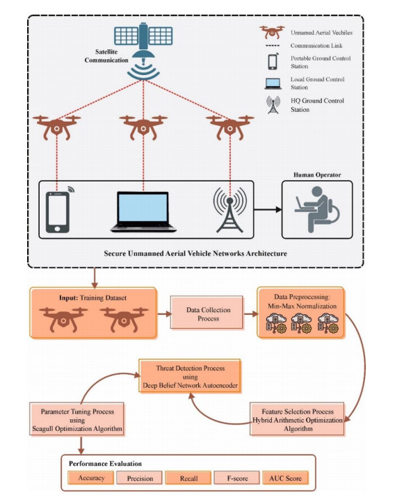
Securing Unmanned Aerial Vehicle (UAV) systems is vital to safeguard the processes involved in operating the drones. This involves the execution of robust communication encryption processes to defend the data exchanged between the UAVs and ground control stations. Intrusion detection, powered by Deep Learning (DL) techniques such as Convolutional Neural Networks (CNN), allows the classification and identification of potential attacks or illegal objects in the operational region of the drone, thus distinguishing them from the routine basics. The current research work offers a new Hybrid Arithmetic Optimizer Algorithm with DL method for Secure Unmanned Aerial Vehicle Network (HAOADL-UAVN) model. The purpose of the proposed HAOADL-UAVN technique is to secure the communication that occurs in UAV networks via threat detection. At the primary level, the network data is normalized through min-max normalization approach in order to scale the input dataset into a useful format. The HAOA is used to select a set of optimal features. Next, the security is attained via Deep Belief Network Autoencoder (DBN-AE)-based threat detection. At last, the hyperparameter choice of the DBN-AE method is implemented using the Seagull Optimization Algorithm (SOA). A huge array of simulations was conducted using the benchmark datasets to demonstrate the improved performance of the proposed HAOADL-UAVN algorithm. The comprehensive results underline the supremacy of the HAOADL-UAVN methodology under distinct evaluation metrics.

| [1] |
T. Alladi, V. Kohli, V. Chamola, F. R. Yu, A deep learning-based misbehavior classification scheme for intrusion detection in cooperative intelligent transportation systems, Digit. Commun. Netw., 9 (2023), 1113–1122. https://doi.org/10.1016/j.dcan.2022.06.018 doi: 10.1016/j.dcan.2022.06.018

|
| [2] | K. H. Park, E. Park, H. K. Kim, Unsupervised intrusion detection system for unmanned aerial vehicle with less labeling effort. In: Information security applications: 21st international conference, Springer, Cham. 2020, 45–58. https://doi.org/10.1007/978-3-030-65299-9_4 |
| [3] | S. Jeong, E. Park, K. U. Seo, J. Do Yoo, H. K. Kim, MUVIDS: false MAVLink injection attack detection in communication for unmanned vehicles. In: Workshop on automotive and autonomous vehicle security (AutoSec), 2021. https://doi.org/10.14722/autosec.2021.23036 |
| [4] |
D. Basavaraj, S. Tayeb, Towards a lightweight intrusion detection framework for in-vehicle networks, J. Sensor Actuator Netw., 11 (2022), 6. https://doi.org/10.3390/jsan11010006 doi: 10.3390/jsan11010006
|
| [5] |
P. Mansourian, N. Zhang, A. Jaekel, M. Kneppers, Deep learning-based anomaly detection for connected autonomous vehicles using spatiotemporal information, IEEE T. Intell. Transp. Syst., 24 (2023), 16006–16017. https://doi.org/10.1109/TITS.2023.3286611 doi: 10.1109/TITS.2023.3286611
|
| [6] |
L. Yang, A. Moubayed, A. Shami, MTH-IDS: A multitiered hybrid intrusion detection system for internet of vehicles, IEEE Internet Things J., 9 (2022), 616–632. https://doi.org/10.1109/JIOT.2021.3084796 doi: 10.1109/JIOT.2021.3084796
|
| [7] | N. Vanitha, P. Ganapathi, Traffic analysis of UAV networks using enhanced deep feed forward neural networks (EDFFNN). In: Handbook of research on machine and deep learning applications for cyber security. 2020. https://doi.org/10.4018/978-1-5225-9611-0.ch011 |
| [8] |
S. Aziz, M. T. Faiz, A. M. Adeniyi, K. H. Loo, K. N. Hasan, L. Xu, et al., Anomaly detection in the internet of vehicular networks using explainable neural networks (xnn), Mathematics, 10 (2022), 1267. https://doi.org/10.3390/math10081267 doi: 10.3390/math10081267
|
| [9] |
S. Anbalagan, G. Raja, S. Gurumoorthy, R. D. Suresh, K. Dev, ⅡDS: Intelligent intrusion detection system for sustainable development in autonomous vehicles, IEEE T. Intell. Transp. Syst., 24 (2023), 15866–15875. https://doi.org/10.1109/TITS.2023.3271768 doi: 10.1109/TITS.2023.3271768
|
| [10] |
R. Fotohi, E. Nazemi, F. S. Aliee, An agent-based self-protective method to secure communication between UAVs in unmanned aerial vehicle networks, Veh. Commun., 26 (2020), 100267. https://doi.org/10.1016/j.vehcom.2020.100267 doi: 10.1016/j.vehcom.2020.100267
|
| [11] |
F. Kateb, M. Ragab, Archimedes optimization with deep learning based aerial image classification for cybersecurity enabled UAV networks, Comput. Syst. Sci. Eng., 47 (2023), 2171–2185. https://doi.org/10.32604/csse.2023.039931 doi: 10.32604/csse.2023.039931
|
| [12] |
M. A. Sayeed, R. Kumar, V. Sharma, Safeguarding unmanned aerial systems: An approach for identifying malicious aerial nodes, IET Commun., 14 (2020), 3000–3012. https://doi.org/10.1049/iet-com.2020.0073 doi: 10.1049/iet-com.2020.0073
|
| [13] |
J. Tao, T. Han, R. Li, Deep-reinforcement-learning-based intrusion detection in aerial computing networks, IEEE Netw., 35 (2021), 66–72. https://doi.org/10.1109/MNET.011.2100068 doi: 10.1109/MNET.011.2100068
|
| [14] |
A. Masadeh, M. Alhafnawi, H. A. B. Salameh, A. Musa, Y. Jararweh, Reinforcement learning-based security/safety uav system for intrusion detection under dynamic and uncertain target movement, IEEE T. Eng. Manage., 2022, 1–11. https://doi.org/10.1109/TEM.2022.3165375 doi: 10.1109/TEM.2022.3165375
|
| [15] |
R. Kumar, P. Kumar, R. Tripathi, G. P. Gupta, T. R. Gadekallu, G. Srivastava, SP2F: A secured privacy-preserving framework for smart agricultural Unmanned Aerial Vehicles, Comput. Netw., 187 (2021), 107819. https://doi.org/10.1016/j.comnet.2021.107819 doi: 10.1016/j.comnet.2021.107819
|
| [16] |
L. Almutairi, R. Daniel, S. Khasimbee, E. L. Lydia, S. Acharya, H. Kim, Quantum dwarf mongoose optimization with ensemble deep learning based intrusion detection in cyber-physical systems, IEEE Access, 11 (2023), 66828–66837. https://doi.org/10.1109/ACCESS.2023.3287896 doi: 10.1109/ACCESS.2023.3287896
|
| [17] | I. U. Khan, A. Abdollahi, M. A. Khan, I. Uddin, I. Ullah, Securing against DoS/DDoS attacks in internet of flying things using experience-based deep learning algorithm, 2021. (Preprint) https://doi.org/10.21203/rs.3.rs-271920/v1 |
| [18] |
Q. Abu Al-Haija, A. Al Badawi, High-performance intrusion detection system for networked UAVs via deep learning, Neural Comput. Appl., 34 (2022), 10885–10900. https://doi.org/10.1007/s00521-022-07015-9 doi: 10.1007/s00521-022-07015-9
|
| [19] |
M. S. Minu, R. Aroul Canessane, S. S. Subashka Ramesh, Optimal squeeze net with deep neural network-based arial image classification model in Unmanned Aerial Vehicles, Traitement du Signal, 39 (2022), 275–281. https://doi.org/10.18280/ts.390128 doi: 10.18280/ts.390128
|
| [20] |
J. Tian, B Wang, R. Guo, Z. Wang, K. Cao, X. Wang, Adversarial attacks and defenses for deep-learning-based unmanned aerial vehicles, IEEE Internet Things J., 9 (2021), 22399–22409. https://doi.org/10.1109/JIOT.2021.3111024 doi: 10.1109/JIOT.2021.3111024
|
| [21] |
V. F. S. Francelin, J. Daniel, S. Velliangiri, Intelligent agent and optimization‐based deep residual network to secure communication in UAV network, Int. J. Intell. Syst., 37 (2022), 5508–5529. https://doi.org/10.1002/int.22800 doi: 10.1002/int.22800
|
| [22] |
H. Zhang, J. Xue, Q. Wang, Y. Li, A security optimization scheme for data security transmission in UAV-assisted edge networks based on federal learning, Ad Hoc Netw., 150 (2023), 103277. https://doi.org/10.1016/j.adhoc.2023.103277 doi: 10.1016/j.adhoc.2023.103277
|
| [23] |
A. M. Elshewey, M. Y. Shams, N. El-Rashidy, A. M. Elhady, S. M. Shohieb, Z. Tarek, Bayesian optimization with support vector machine model for Parkinson disease classification, Sensors, 23 (2023), 2085. https://doi.org/10.3390/s23042085 doi: 10.3390/s23042085
|
| [24] |
M. Stankovic, J. Gavrilovic, D. Jovanovic, M. Zivkovic, M. Antonijevic, N. Bacanin, et al., Tuning multi-layer perceptron by hybridized arithmetic optimization algorithm for healthcare 4.0, Procedia Comput. Sci., 215 (2022), 51–60. https://doi.org/10.1016/j.procs.2022.12.006 doi: 10.1016/j.procs.2022.12.006
|
| [25] |
H. Al-Khazraji, A. R. Nasser, A. M. Hasan, A. K. Al Mhdawi, H. Al-Raweshidy, A. J. Humaidi, Aircraft engines remaining useful life prediction based on a hybrid model of autoencoder and deep belief network, IEEE Access, 10 (2022), 82156–82163. https://doi.org/10.1109/ACCESS.2022.3188681 doi: 10.1109/ACCESS.2022.3188681
|
| [26] |
P. Krishnadoss, V. K. Poornachary, P. Krishnamoorthy, L. Shanmugam, Improvised seagull optimization algorithm for scheduling tasks in heterogeneous cloud environment, Comput. Mater. Con., 74 (2023), 2461–2478. https://doi.org/10.32604/cmc.2023.031614 doi: 10.32604/cmc.2023.031614
|
| [27] |
N. Moustafa, A new distributed architecture for evaluating AI-based security systems at the edge: Network TON_IoT datasets, Sustain. Cities Soc., 72 (2021), 102994. https://doi.org/10.1016/j.scs.2021.102994 doi: 10.1016/j.scs.2021.102994
|
| [28] |
R. A. Ramadan, A. H. Emara, M. Al-Sarem, M. Elhamahmy, Internet of drones intrusion detection using deep learning, Electronics, 10 (2021), 2633. https://doi.org/10.3390/electronics10212633 doi: 10.3390/electronics10212633
|
| [29] |
L. Kou, S. Ding, T. Wu, W. Dong, Y. Yin, An intrusion detection model for drone communication network in SDN environment, Drones, 6 (2022), 342. https://doi.org/10.3390/drones6110342 doi: 10.3390/drones6110342
|


Figures(12) / Tables(4)

Sultanah M. Alshammari, Nofe A. Alganmi, Mohammed H. Ba-Aoum, Sami Saeed Binyamin, Abdullah AL-Malaise AL-Ghamdi, Mahmoud Ragab. Hybrid arithmetic optimization algorithm with deep learning model for secure Unmanned Aerial Vehicle networks[J]. AIMS Mathematics, 2024, 9(3): 7131-7151. doi: 10.3934/math.2024348


 DownLoad: