The land cover classification process, accomplished through Remote Sensing Imagery (RSI), exploits advanced Machine Learning (ML) approaches to classify different types of land cover within the geographical area, captured by the RS method. The model distinguishes various types of land cover under different classes, such as agricultural fields, water bodies, urban areas, forests, etc. based on the patterns present in these images. The application of Deep Learning (DL)-based land cover classification technique in RSI revolutionizes the accuracy and efficiency of land cover mapping. By leveraging the abilities of Deep Neural Networks (DNNs) namely, Convolutional Neural Networks (CNN) or Recurrent Neural Networks (RNN), the technology can autonomously learn spatial and spectral features inherent to the RSI. The current study presents an Improved Sand Cat Swarm Optimization with Deep Learning-based Land Cover Classification (ISCSODL-LCC) approach on the RSIs. The main objective of the proposed method is to efficiently classify the dissimilar land cover types within the geographical area, pictured by remote sensing models. The ISCSODL-LCC technique utilizes advanced machine learning methods by employing the Squeeze-Excitation ResNet (SE-ResNet) model for feature extraction and the Stacked Gated Recurrent Unit (SGRU) mechanism for land cover classification. Since 'manual hyperparameter tuning' is an erroneous and laborious task, the hyperparameter selection is accomplished with the help of the Reptile Search Algorithm (RSA). The simulation analysis was conducted upon the ISCSODL-LCC model using two benchmark datasets and the results established the superior performance of the proposed model. The simulation values infer better outcomes of the ISCSODL-LCC method over other techniques with the maximum accuracy values such as 97.92% and 99.14% under India Pines and Pavia University datasets, respectively.
Citation: Abdelwahed Motwake, Aisha Hassan Abdalla Hashim, Marwa Obayya, Majdy M. Eltahir. Enhancing land cover classification in remote sensing imagery using an optimal deep learning model[J]. AIMS Mathematics, 2024, 9(1): 140-159. doi: 10.3934/math.2024009
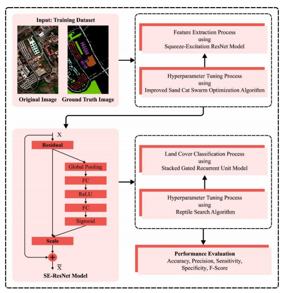
The land cover classification process, accomplished through Remote Sensing Imagery (RSI), exploits advanced Machine Learning (ML) approaches to classify different types of land cover within the geographical area, captured by the RS method. The model distinguishes various types of land cover under different classes, such as agricultural fields, water bodies, urban areas, forests, etc. based on the patterns present in these images. The application of Deep Learning (DL)-based land cover classification technique in RSI revolutionizes the accuracy and efficiency of land cover mapping. By leveraging the abilities of Deep Neural Networks (DNNs) namely, Convolutional Neural Networks (CNN) or Recurrent Neural Networks (RNN), the technology can autonomously learn spatial and spectral features inherent to the RSI. The current study presents an Improved Sand Cat Swarm Optimization with Deep Learning-based Land Cover Classification (ISCSODL-LCC) approach on the RSIs. The main objective of the proposed method is to efficiently classify the dissimilar land cover types within the geographical area, pictured by remote sensing models. The ISCSODL-LCC technique utilizes advanced machine learning methods by employing the Squeeze-Excitation ResNet (SE-ResNet) model for feature extraction and the Stacked Gated Recurrent Unit (SGRU) mechanism for land cover classification. Since 'manual hyperparameter tuning' is an erroneous and laborious task, the hyperparameter selection is accomplished with the help of the Reptile Search Algorithm (RSA). The simulation analysis was conducted upon the ISCSODL-LCC model using two benchmark datasets and the results established the superior performance of the proposed model. The simulation values infer better outcomes of the ISCSODL-LCC method over other techniques with the maximum accuracy values such as 97.92% and 99.14% under India Pines and Pavia University datasets, respectively.

| [1] |
T. Kwak, Y. Kim, Semi-supervised land cover classification of remote sensing imagery using CycleGAN and EfficientNet, KSCE J. Civ. Eng., 27 (2023), 1760–1773. https://doi.org/10.1007/s12205-023-2285-0 doi: 10.1007/s12205-023-2285-0

|
| [2] |
T. He, S. Wang, Multi-spectral remote sensing land-cover classification based on deep learning methods, J. Supercomput., 77 (2021), 2829–2843. https://doi.org/10.1007/s11227-020-03377-w doi: 10.1007/s11227-020-03377-w
|
| [3] |
L. Wang, J. Wang, Z. Liu, J. Zhu, F. Qin, Evaluation of a deep-learning model for multispectral remote sensing of land use and crop classification, Crop. J., 10 (2022), 1435–1451. https://doi.org/10.1016/j.cj.2022.01.009 doi: 10.1016/j.cj.2022.01.009
|
| [4] |
A. Tzepkenlis, K. Marthoglou, N. Grammalidis, Efficient deep semantic segmentation for land cover classification using sentinel imagery, Remote Sens., 15 (2023), 2027. https://doi.org/10.3390/rs15082027 doi: 10.3390/rs15082027
|
| [5] |
Y. Li, Y. Zhou, Y. Zhang, L. Zhong, J. Wang, J. Chen, DKDFN: Domain knowledge-guided deep collaborative fusion network for multimodal unitemporal remote sensing land cover classification, ISPRS J. Photogramm. Remote Sens., 186 (2022), 170–189. https://doi.org/10.1016/j.isprsjprs.2022.02.013 doi: 10.1016/j.isprsjprs.2022.02.013
|
| [6] |
L. Bergamasco, F. Bovolo, L. Bruzzone, A dual-branch deep learning architecture for multisensor and multitemporal remote sensing semantic segmentation, IEEE J. STARS, 16 (2023), 2147–2162. https://doi.org/10.1109/JSTARS.2023.3243396 doi: 10.1109/JSTARS.2023.3243396
|
| [7] |
X. Yuan, Z. Chen, N. Chen, J. Gong, Land cover classification based on the PSPNet and superpixel segmentation methods with high spatial resolution multispectral remote sensing imagery, J. Appl. Remote Sens., 15 (2021), 034511. https://doi.org/10.1117/1.JRS.15.034511 doi: 10.1117/1.JRS.15.034511
|
| [8] | J. Yan, J. Liu, L. Wang, D. Liang, Q. Cao, W. Zhang, et al., Land-cover classification with time-series remote sensing images by complete extraction of multiscale timing dependence, IEEE J. STARS, 15 (2022), 1953–1967. https://doi.org/10.1109/JSTARS.2022.3150430 |
| [9] | J. Kim, Y. Song, W. K. Lee, Accuracy analysis of multi-series phenological landcover classification using U-Net-based deep learning model–Focusing on the Seoul, Republic of Korea–, Korean J. Remote Sens., 37 (2021), 409–418. https://doi.org/10.7780/kjrs.2020.37.3.4 |
| [10] |
V. Yaloveha, A. Podorozhniak, H. Kuchuk, Convolutional neural network hyperparameter optimization applied to land cover classification, Radioelectron. Comput. Syst., 2022,115–128. https://doi.org/10.32620/reks.2022.1.09 doi: 10.32620/reks.2022.1.09
|
| [11] |
A. Temenos, N. Temenos, M. Kaselimi, A. Doulamis, N. Doulamis, Interpretable deep learning framework for land use and land cover classification in remote sensing using SHAP, IEEE Geosci. Remote Sens. Lett., 20 (2023), 8500105. https://doi.org/10.1109/LGRS.2023.3251652 doi: 10.1109/LGRS.2023.3251652
|
| [12] | X. Cheng, X. He, M. Qiao, P. Li, S. Hu, P. Chang, et al., Enhanced contextual representation with deep neural networks for land cover classification based on remote sensing images, Int. J. Appl. Earth Obse., 107 (2022), 102706. https://doi.org/10.1016/j.jag.2022.102706 |
| [13] |
B. Ekim, E. Sertel, Deep neural network ensembles for remote sensing land cover and land use classification, Int. J. Digit. Earth, 14 (2021), 1868–1881. https://doi.org/10.1080/17538947.2021.1980125 doi: 10.1080/17538947.2021.1980125
|
| [14] |
V. N. Vinaykumar, J. A. Babu, J. Frnda, Optimal guidance whale optimization algorithm and hybrid deep learning networks for land use land cover classification, EURASIP J. Adv. Signal Process., 2023 (2023), 13. https://doi.org/10.1186/s13634-023-00980-w doi: 10.1186/s13634-023-00980-w
|
| [15] |
M. Luo, S. Ji, Cross-spatiotemporal land-cover classification from VHR remote sensing images with deep learning based domain adaptation, ISPRS J. Photogramm. Remote Sens., 191 (2022), 105–128. https://doi.org/10.1016/j.isprsjprs.2022.07.011 doi: 10.1016/j.isprsjprs.2022.07.011
|
| [16] |
W. Zhou, C. Persello, A. Stein, Building usage classification using a transformer-based multimodal deep learning method, 2023 Joint Urban Remote Sensing Event (JURSE), 2023. https://doi.org/10.1109/JURSE57346.2023.10144168 doi: 10.1109/JURSE57346.2023.10144168
|
| [17] |
G. P. Joshi, F. Alenezi, G. Thirumoorthy, A. K. Dutta, J. You, Ensemble of deep learning-based multimodal remote sensing image classification model on unmanned aerial vehicle networks, Mathematics, 9 (2021), 2984. https://doi.org/10.3390/math9222984 doi: 10.3390/math9222984
|
| [18] |
R. Li, S. Zheng, C. Duan, L. Wang, C. Zhang, Land cover classification from remote sensing images based on multi-scale fully convolutional network, Geo-Spat. Inf Sci., 25 (2022), 278–294. https://doi.org/10.1080/10095020.2021.2017237 doi: 10.1080/10095020.2021.2017237
|
| [19] |
A. Tariq, F. Mumtaz, Modeling spatio-temporal assessment of land use land cover of Lahore and its impact on land surface temperature using multi-spectral remote sensing data, Environ. Sci. Pollut. Res., 30 (2022), 23908–23924. https://doi.org/10.1007/s11356-022-23928-3 doi: 10.1007/s11356-022-23928-3
|
| [20] | A. Tariq, J. Yan, F. Mumtaz, Land change modeler and CA-Markov chain analysis for land use land cover change using satellite data of Peshawar, Pakistan, Phys. Chem. Earth Parts A/B/C, 128 (2022), 103286. |
| [21] |
A. Tariq, F. Mumtaz, M. Majeed, X. Zeng, Spatio-temporal assessment of land use land cover based on trajectories and cellular automata Markov modelling and its impact on land surface temperature of Lahore district Pakistan, Environ. Monit. Assess., 195 (2023), 114. https://doi.org/10.1007/s10661-022-10738-w doi: 10.1007/s10661-022-10738-w
|
| [22] | A. Tariq, H. Shu, CA-Markov chain analysis of seasonal land surface temperature and land use land cover change using optical multi-temporal satellite data of Faisalabad, Pakistan, Remote Sens., 12 (2020), 3402. https://doi.org/10.3390/rs12203402 |
| [23] |
T. Chen, H. Qin, X. Li, W. Wan, W. Yan, A Non-Intrusive Load Monitoring Method Based on Feature Fusion and SE-ResNet, Electronics, 12 (2023), 1909. https://doi.org/10.3390/electronics12081909 doi: 10.3390/electronics12081909
|
| [24] | H. Long, Y. He, Y. Xu, C. You, D. Zeng, H. Lu, Optimal allocation research of distribution network with DGs and SCs by improved sand cat swarm optimization algorithm, IAENG Int. J. Comput. Sci., 2023. |
| [25] |
A. Al Hamoud, A. Hoenig, K. Roy, Sentence subjectivity analysis of a political and ideological debate dataset using LSTM and BiLSTM with attention and GRU models, J. King Saud Univ.-Com., 34 (2022), 7974–7987. https://doi.org/10.1016/j.jksuci.2022.07.014 doi: 10.1016/j.jksuci.2022.07.014
|
| [26] |
L. Kong, H. Liang, G. Liu, S. Liu, Research on wind turbine fault detection based on the fusion of ASL-CatBoost and TtRSA, Sensors, 23 (2023), 6741. https://doi.org/10.3390/s23156741 doi: 10.3390/s23156741
|
| [27] |
S. Rajalakshmi, S. Nalini, A. Alkhayyat, R. Q. Malik, Hyperspectral remote sensing image classification using improved metaheuristic with deep learning, Comput. Syst. Sci. Eng., 46 (2023), 1673–1688. https://doi.org/10.32604/csse.2023.034414 doi: 10.32604/csse.2023.034414
|


Figures(8) / Tables(6)

Abdelwahed Motwake, Aisha Hassan Abdalla Hashim, Marwa Obayya, Majdy M. Eltahir. Enhancing land cover classification in remote sensing imagery using an optimal deep learning model[J]. AIMS Mathematics, 2024, 9(1): 140-159. doi: 10.3934/math.2024009


 DownLoad: