Advancements in remote sensing: Harnessing the power of artificial intelligence for scene image classification

Alaa O. Khadidos; Alaa O. Khadidos

doi:10.3934/math.2024500

AIMS Mathematics

2024, Volume 9, Issue 4: 10235-10254. doi: 10.3934/math.2024500

Previous Article Next Article

Research article Special Issues

Advancements in remote sensing: Harnessing the power of artificial intelligence for scene image classification

Alaa O. Khadidos ^{1,2
,
,}

1.
Associate Professor, Department of Information Systems, Faculty of Computing and Information Technology, King Abdulaziz University, Jeddah, Saudi Arabia
2.
Center of Research Excellence in Artificial Intelligence and Data Science, King Abdulaziz University, Jeddah, Saudi Arabia

Received: 15 November 2023 Revised: 24 February 2024 Accepted: 27 February 2024 Published: 14 March 2024
MSC : 68M11, 68M25, 68T07, 68W1

The Remote Sensing Scene Image Classification (RSSIC) procedure is involved in the categorization of the Remote Sensing Images (RSI) into sets of semantic classes depending upon the content and this procedure plays a vital role in extensive range of applications, like environment monitoring, urban planning, vegetation mapping, natural hazards' detection and geospatial object detection. The RSSIC procedure exploits Artificial Intelligence (AI) technology, mostly Machine Learning (ML) techniques, for automatic analysis and categorization of the content, present in these images. The purpose is to recognize and differentiate the land cover classes or features in the scene, namely crops, forests, buildings, water bodies, roads, and other natural and man-made structures. RSSIC, using Deep Learning (DL) techniques, has attracted a considerable attention and accomplished important breakthroughs, thanks to the great feature learning abilities of the Deep Neural Networks (DNNs). In this aspect, the current study presents the White Shark Optimizer with DL-driven RSSIC (WSODL-RSSIC) technique. The presented WSODL-RSSIC technique mainly focuses on detection and classification of the remote sensing images under various class labels. In the WSODL-RSSIC technique, the deep Convolutional Neural Network (CNN)-based ShuffleNet model is used to produce the feature vectors. Moreover, the Deep Multilayer Neural network (DMN) classifiers are utilized for recognition and classification of the remote sensing images. Furthermore, the WSO technique is used to optimally adjust the hyperparameters of the DMN classifier. The presented WSODL-RSSIC method was simulated for validation using the remote-sensing image databases. The experimental outcomes infer that the WSODL-RSSIC model achieved improved results in comparison with the current approaches under different evaluation metrics.
- remote sensing images,
- artificial intelligence,
- white shark optimizer,
- scene classification,
- deep learning
Citation: Alaa O. Khadidos. Advancements in remote sensing: Harnessing the power of artificial intelligence for scene image classification[J]. AIMS Mathematics, 2024, 9(4): 10235-10254. doi: 10.3934/math.2024500

Related Papers:

Abstract

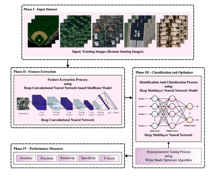
The Remote Sensing Scene Image Classification (RSSIC) procedure is involved in the categorization of the Remote Sensing Images (RSI) into sets of semantic classes depending upon the content and this procedure plays a vital role in extensive range of applications, like environment monitoring, urban planning, vegetation mapping, natural hazards' detection and geospatial object detection. The RSSIC procedure exploits Artificial Intelligence (AI) technology, mostly Machine Learning (ML) techniques, for automatic analysis and categorization of the content, present in these images. The purpose is to recognize and differentiate the land cover classes or features in the scene, namely crops, forests, buildings, water bodies, roads, and other natural and man-made structures. RSSIC, using Deep Learning (DL) techniques, has attracted a considerable attention and accomplished important breakthroughs, thanks to the great feature learning abilities of the Deep Neural Networks (DNNs). In this aspect, the current study presents the White Shark Optimizer with DL-driven RSSIC (WSODL-RSSIC) technique. The presented WSODL-RSSIC technique mainly focuses on detection and classification of the remote sensing images under various class labels. In the WSODL-RSSIC technique, the deep Convolutional Neural Network (CNN)-based ShuffleNet model is used to produce the feature vectors. Moreover, the Deep Multilayer Neural network (DMN) classifiers are utilized for recognition and classification of the remote sensing images. Furthermore, the WSO technique is used to optimally adjust the hyperparameters of the DMN classifier. The presented WSODL-RSSIC method was simulated for validation using the remote-sensing image databases. The experimental outcomes infer that the WSODL-RSSIC model achieved improved results in comparison with the current approaches under different evaluation metrics.

References

[1]	S. Thirumaladevi, K. V. Swamy, M. Sailaja, Remote sensing image scene classification by transfer learning to augment the accuracy, Meas. Sens., 25 (2023), 100645. https://doi.org/10.1016/j.measen.2022.100645 doi: 10.1016/j.measen.2022.100645
[2]	M. Ragab, Multi-label scene classification on remote sensing imagery using modified Dingo optimizer with deep learning, IEEE Access, 12 (2023), 11879–11886. https://doi.org/10.1109/ACCESS.2023.3344773 doi: 10.1109/ACCESS.2023.3344773
[3]	P. Wang, H. Zhao, Z. Yang, Q. Jin, Y. Wu, P. Xia, et al., Fast tailings pond mapping exploiting large scene remote sensing images by coupling scene classification and sematic segmentation models, Remote Sens., 15 (2023), 327. https://doi.org/10.3390/rs15020327 doi: 10.3390/rs15020327
[4]	M. Ye, N. Ruiwen, Z. Chang, G. He, H. Tianli, L. Shijun, et al., A lightweight model of VGG-16 for remote sensing image classification, IEEE J-STARS, 14 (2021), 6916–6922. https://doi.org/10.1109/JSTARS.2021.3090085 doi: 10.1109/JSTARS.2021.3090085
[5]	M. Ragab, H. A. Abdushkour, A. O. Khadidos, A. M. Alshareef, K. H. Alyoubi, A. O. Khadidos, Improved deep learning-based vehicle detection for urban applications using remote sensing imagery, Remote Sens., 15 (2023), 4747. https://doi.org/10.3390/rs15194747 doi: 10.3390/rs15194747
[6]	A. A. Aljabri, A. Alshanqiti, A. B. Alkhodre, A. Alzahem, A. Hagag, Extracting feature fusion and co-saliency clusters using transfer learning techniques for improving remote sensing scene classification, Optik, 273 (2023), 170408. https://doi.org/10.1016/j.ijleo.2022.170408 doi: 10.1016/j.ijleo.2022.170408
[7]	X. Tang, W. Lin, J. Ma, X. Zhang, F Liu, L. Jiao, Class-level prototype guided multiscale feature learning for remote sensing scene classification with limited labels, IEEE T. Geosci. Remote Sens., 60 (2022), 5622315. https://doi.org10.1109/TGRS.2022.3169835 doi: 10.1109/TGRS.2022.3169835
[8]	M. N. Akhtar, E. Ansari, S. S. N. Alhady, E. A. Bakar, Leveraging on advanced remote sensing-and artificial intelligence-based technologies to manage palm oil plantation for current global scenario: A review, Agriculture, 13 (2023), 504. https://doi.org/10.3390/agriculture13020504 doi: 10.3390/agriculture13020504
[9]	C. Peng, Y. Li, R. Shang, L. Jiao, RSBNet: One-shot neural architecture search for a backbone network in remote sensing image recognition, Neurocomputing, 537 (2023), 110–127. https://doi.org/10.1016/j.neucom.2023.03.046 doi: 10.1016/j.neucom.2023.03.046
[10]	X. Huang, Y. Sun, S. Feng, Y. Ye, X. Li, Better visual interpretation for remote sensing scene classification, IEEE Geosci. Remote Sens. Lett., 19 (2022), 6504305. https://doi.org/10.1109/LGRS.2021.3132920 doi: 10.1109/LGRS.2021.3132920
[11]	Y. Sun, W. Zheng, HRNet-and PSPNet-based multiband semantic segmentation of remote sensing images, Neural Comput. Appl., 35 (2023), 8667–8675. https://doi.org/10.1007/s00521-022-07737-w doi: 10.1007/s00521-022-07737-w
[12]	H. Sun, Y. Lin, Q. Zou, S. Song, J. Fang, H. Yu, Convolutional neural networks based remote sensing scene classification under clear and cloudy environments, In: 2021 IEEE/CVF International Conference on Computer Vision Workshops (ICCVW), 2021,713–720. https://doi.org/10.1109/ICCVW54120.2021.00085
[13]	W. Miao, J. Geng, W. Jiang, Semi-supervised remote-sensing image scene classification using representation consistency Siamese network, IEEE T. Geosci. Remote Sens., 60 (2022), 5616614. https://doi.org/10.1109/TGRS.2022.3140485 doi: 10.1109/TGRS.2022.3140485
[14]	X. Xu, Y. Chen, J. Zhang, Y. Chen, P. Anandhan, A. Manickam, A novel approach for scene classification from remote sensing images using deep learning methods, Eur. J. Remote Sens., 54 (2021), 383–395. https://doi.org/10.1080/22797254.2020.1790995 doi: 10.1080/22797254.2020.1790995
[15]	X. Cheng, H. Lei, Remote sensing scene image classification based on mmsCNN–HMM with stacking ensemble model, Remote Sens., 14 (2022), 4423. https://doi.org/10.3390/rs14174423 doi: 10.3390/rs14174423
[16]	A. M. Hilal, F. N. Al-Wesabi, K. J. Alzahrani, M. Al Duhayyim, M. A. Hamza, M. Rizwanullah, et al., Deep transfer learning based fusion model for environmental remote sensing image classification model, Eur. J. Remote Sens., 55 (2022), 12–23. https://doi.org/10.1080/22797254.2021.2017799 doi: 10.1080/22797254.2021.2017799
[17]	G. Zhang, W. Xu, W. Zhao, C. Huang, E. N. Yk, Y. Chen, et al., A multiscale attention network for remote sensing scene images classification, IEEE J-STARS, 14 (2021), 9530–9545. https://doi.org/10.1109/JSTARS.2021.3109661 doi: 10.1109/JSTARS.2021.3109661
[18]	C. Xu, G. Zhu, J. Shu, A lightweight and robust lie group-convolutional neural networks joint representation for remote sensing scene classification, IEEE T. Geoscie. Remote Sens., 60 (2022), 5501415. https://doi.org/10.1109/TGRS.2020.3048024 doi: 10.1109/TGRS.2020.3048024
[19]	J. Wang, W. Li, M. Zhang, R. Tao, J. Chanussot, Remote sensing scene classification via multi-stage self-guided separation network, IEEE T. Geosci. Remote Sens., 61 (2023), 5615312. https://doi.org/10.1109/TGRS.2023.3295797 doi: 10.1109/TGRS.2023.3295797
[20]	M. Ragab, Leveraging mayfly optimization with deep learning for secure remote sensing scene image classification, Comput. Electr. Eng., 108 (2023), 108672. https://doi.org/10.1016/j.compeleceng.2023.108672 doi: 10.1016/j.compeleceng.2023.108672
[21]	J. Geng, B. Xue, W. Jiang, Foreground-background contrastive learning for few-shot remote sensing image scene classification, IEEE T. Geosci. Remote Sens., 61 (2023), 5614112. https://doi.org/10.1109/TGRS.2023.3290794 doi: 10.1109/TGRS.2023.3290794
[22]	L. Huang, W. Zhao, A. W. C. Liew, Y. You, An evidential combination method with multi-color spaces for remote sensing image scene classification, Inform. Fusion, 93 (2023), 209–226. https://doi.org/10.1016/j.inffus.2022.12.025 doi: 10.1016/j.inffus.2022.12.025
[23]	Y. Zhao, J. Liu, J. Yang, Z. Wu, EMSCNet: Efficient multisample contrastive network for remote sensing image scene classification, IEEE T. Geosci. Remote Sens., 61 (2023), 5605814. https://doi.org/10.1109/TGRS.2023.3262840 doi: 10.1109/TGRS.2023.3262840
[24]	D. Singh, Y. S. Taspinar, R. Kursun, I. Cinar, M. Koklu, I. A. Ozkan, et al., Classification and analysis of pistachio species with pre-trained deep learning models, Electronics, 11 (2022), 981. https://doi.org/10.3390/electronics11070981 doi: 10.3390/electronics11070981
[25]	X. Zhang, X. Zhou, M. Lin, J. Sun, Shufflenet: An extremely efficient convolutional neural network for mobile devices. In: 2018 IEEE/CVF Conference on Computer Vision and Pattern Recognition, 2018, 6848–6856. https://doi.org/10.1109/CVPR.2018.00716
[26]	M. Khashei, F. Chahkoutahi, N. Bakhtiarvand, A novel discrete deep learning-based intelligent methodology for energy consumption classification, Energy Rep., 9 (2023), 4861–4871. https://doi.org/10.1016/j.egyr.2023.04.006 doi: 10.1016/j.egyr.2023.04.006
[27]	A. Fathy, D. Yousri, A. G. Alharbi, M. A. A bdelkareem, A new hybrid white shark and whale optimization approach for estimating the Li-Ion battery model parameters, Sustainability, 15 (2023), 5667. https://doi.org/10.3390/su15075667 doi: 10.3390/su15075667
[28]	UC Merced land use dataset, Available from: http://weegee.vision.ucmerced.edu/datasets/landuse.html.

Reader Comments

Your name:*

Email:*
© 2024 the Author(s), licensee AIMS Press. This is an open access article distributed under the terms of the Creative Commons Attribution License (http://creativecommons.org/licenses/by/4.0)