Mathematical formulations are crucial in understanding the dynamics of disease spread within a community. The objective of this research is to investigate the SEIR model of SARS-COVID-19 (C-19) with the inclusion of vaccinated effects for low immune individuals. A mathematical model is developed by incorporating vaccination individuals based on a proposed hypothesis. The fractal-fractional operator (FFO) is then used to convert this model into a fractional order. The newly developed SEVIR system is examined in both a qualitative and quantitative manner to determine its stable state. The boundedness and uniqueness of the model are examined to ensure reliable findings, which are essential properties of epidemic models. The global derivative is demonstrated to verify the positivity with linear growth and Lipschitz conditions for the rate of effects in each sub-compartment. The system is investigated for global stability using Lyapunov first derivative functions to assess the overall impact of vaccination. In fractal-fractional operators, fractal represents the dimensions of the spread of the disease, and fractional represents the fractional ordered derivative operator. We use combine operators to see real behavior of spread as well as control of COVID-19 with different dimensions and continuous monitoring. Simulations are conducted to observe the symptomatic and asymptomatic effects of the corona virus disease with vaccinated measures for low immune individuals, providing insights into the actual behavior of the disease control under vaccination effects. Such investigations are valuable for understanding the spread of the virus and developing effective control strategies based on justified outcomes.
Citation: Huda Alsaud, Muhammad Owais Kulachi, Aqeel Ahmad, Mustafa Inc, Muhammad Taimoor. Investigation of SEIR model with vaccinated effects using sustainable fractional approach for low immune individuals[J]. AIMS Mathematics, 2024, 9(4): 10208-10234. doi: 10.3934/math.2024499
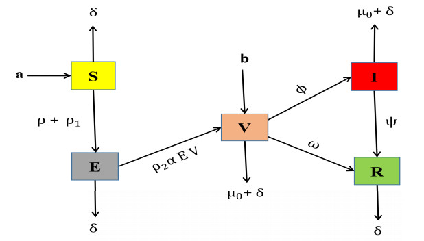
Mathematical formulations are crucial in understanding the dynamics of disease spread within a community. The objective of this research is to investigate the SEIR model of SARS-COVID-19 (C-19) with the inclusion of vaccinated effects for low immune individuals. A mathematical model is developed by incorporating vaccination individuals based on a proposed hypothesis. The fractal-fractional operator (FFO) is then used to convert this model into a fractional order. The newly developed SEVIR system is examined in both a qualitative and quantitative manner to determine its stable state. The boundedness and uniqueness of the model are examined to ensure reliable findings, which are essential properties of epidemic models. The global derivative is demonstrated to verify the positivity with linear growth and Lipschitz conditions for the rate of effects in each sub-compartment. The system is investigated for global stability using Lyapunov first derivative functions to assess the overall impact of vaccination. In fractal-fractional operators, fractal represents the dimensions of the spread of the disease, and fractional represents the fractional ordered derivative operator. We use combine operators to see real behavior of spread as well as control of COVID-19 with different dimensions and continuous monitoring. Simulations are conducted to observe the symptomatic and asymptomatic effects of the corona virus disease with vaccinated measures for low immune individuals, providing insights into the actual behavior of the disease control under vaccination effects. Such investigations are valuable for understanding the spread of the virus and developing effective control strategies based on justified outcomes.

| [1] | I. Podlubny, Fractional differential equations: An introduction to fractional derivatives, fractional differential equations, to methods of their solution and some of their applications, San Diego: Academic Press, 1999. |
| [2] |
A. Atangana, Non validity of index law in fractional calculus: A fractional differential operator with Markovian and non-Markovian properties, Physica A, 505 (2018), 688–706. https://doi.org/10.1016/j.physa.2018.03.056 doi: 10.1016/j.physa.2018.03.056

|
| [3] |
A. K. Golmankhaneh, C. Tunç, Sumudu transform in fractal calculus, Appl. Math. Comput., 350 (2019), 386–401. https://doi.org/10.1016/j.amc.2019.01.025 doi: 10.1016/j.amc.2019.01.025
|
| [4] |
M. Goyal, H. M. Baskonus, A. Prakash, An efficient technique for a time fractional model of lassa hemorrhagic fever spreading in pregnant women, Eur. Phys. J. Plus, 134 (2019), 482. https://doi.org/10.1140/epjp/i2019-12854-0 doi: 10.1140/epjp/i2019-12854-0
|
| [5] |
I. Nesteruk, Statistics based predictions of coronavirus 2019-nCoV spreading in mainland China, Innovative Biosyst. Bioeng., 4 (2020), 13–18. https://doi.org/10.20535/ibb.2020.4.1.195074 doi: 10.20535/ibb.2020.4.1.195074
|
| [6] |
K. Shah, R. U. Din, W. Deebani, P. Kumam, Z. Shah, On nonlinear classical and fractional order dynamical system addressing COVID-19, Results Phys., 24 (2021), 104069. https://doi.org/10.1016/j.rinp.2021.104069 doi: 10.1016/j.rinp.2021.104069
|
| [7] |
A. J. Lotka, Contribution to the theory of periodic reactions, J. Phys. Chem., 14 (1910), 271–274. https://doi.org/10.1021/j150111a004 doi: 10.1021/j150111a004
|
| [8] |
N. S. Goel, S. C. Maitra, E. W. Montroll, On the Volterra and other nonlinear models of interacting populations, Rev. Mod. Phys., 43 (1971), 231. https://doi.org/10.1103/RevModPhys.43.231 doi: 10.1103/RevModPhys.43.231
|
| [9] |
M. M. Khalsaraei, An improvement on the positivity results for 2-stage explicit Runge-Kutta methods, J. Comput. Appl. Math., 235 (2010), 137–143. https://doi.org/10.1016/j.cam.2010.05.020 doi: 10.1016/j.cam.2010.05.020
|
| [10] |
P. Zhou, X. L. Yang, X. G. Wang, B. Hu, L. Zhang, W. Zhang, et al., A pneumonia outbreak associated with a new coronavirus of probable bat origin, Nature, 579 (2020), 270–273. https://doi.org/10.1038/s41586-020-2012-7 doi: 10.1038/s41586-020-2012-7
|
| [11] |
Q. Li, X. Guan, P. Wu, X. Wang, L. Zhou, Y. Tong, et al., Early transmission dynamics in Wuhan, China, of novel coronavirus infected pneumonia, N. Engl. J. Med., 382 (2020), 1199–1207. https://doi.org/10.1056/NEJMoa2001316 doi: 10.1056/NEJMoa2001316
|
| [12] |
I. I. Bogoch, A. Watts, A. Thomas-Bachli, C. Huber, M. U. Kraemer, K. Khan, Pneumonia of unknown aetiology in Wuhan, China: Potential for international spread via commercial air travel, J. Travel Med., 27 (2020), taaa008. https://doi.org/10.1093/jtm/taaa008 doi: 10.1093/jtm/taaa008
|
| [13] |
A. B. Gumel, S. Ruan, T. Day, J. Watmough, F. Brauer, P. Van den Driessche, et al., Modelling strategies for controlling SARS out breaks, Proc. R. Soc. Lond. B, 271 (2004), 2223–2232. https://doi.org/10.1098/rspb.2004.2800 doi: 10.1098/rspb.2004.2800
|
| [14] |
R. Kahn, I. Holmdahl, S. Reddy, J. Jernigan, M. J. Mina, R. B. Slayton, Mathematical modeling to inform vaccination strategies and testing approaches for coronavirus disease 2019 (COVID-19) in nursing homes, Clin. Infect. Dis., 74 (2022), 597–603. https://doi.org/10.1093/cid/ciab517 doi: 10.1093/cid/ciab517
|
| [15] |
J. Mondal, S. Khajanchi, Mathematical modeling and optimal intervention strategies of the COVID-19 outbreak, Nonlinear Dyn., 109 (2022), 177–202. https://doi.org/10.1007/s11071-022-07235-7 doi: 10.1007/s11071-022-07235-7
|
| [16] |
S. Hussain, E. N. Madi, H. Khan, H. Gulzar, S. Etemad, S. Rezapour, et al., On the stochastic modeling of COVID-19 under the environmental white noise, J. Funct. Space, 2022 (2022), 4320865. https://doi.org/10.1155/2022/4320865 doi: 10.1155/2022/4320865
|
| [17] | WHO, Statement on the second meeting of the international health regulations emergency committee regarding the outbreak of novel coronavirus (2019-nCoV), 2020. |
| [18] | J. Page, D. Hinshaw, B. McKay, In hunt for COVID-19 origin, patient zero points to second Wuhan market - the man with the first confirmed infection of the new coronavirus told the WHO team that his parents had shopped there, In: The Wall Street Journal, 2021. |
| [19] |
S. Zhao, H. Chen, Modeling the epidemic dynamics and control of covid-19 outbreak in China, Quant. Biol., 8 (2020), 11–19. https://doi.org/10.1007/s40484-020-0199-0 doi: 10.1007/s40484-020-0199-0
|
| [20] |
C. Rivers, J. P. Chretien, S. Riley, J. A. Pavlin, A. Woodward, D. Brett-Major, et al., Using "outbreak science" to strengthen the use of models during epidemics, Nat. Commun., 10 (2019), 3102. https://doi.org/10.1038/s41467-019-11067-2 doi: 10.1038/s41467-019-11067-2
|
| [21] |
K. Sun, J. Chen, C. Viboud, Early epidemiological analysis of the coronavirus disease 2019 outbreak based on crowd sourced data: A population-level observational study, Lancet Digital Health, 2 (2020), e201–e208. https://doi.org/10.1016/S2589-7500(20)30026-1 doi: 10.1016/S2589-7500(20)30026-1
|
| [22] |
N. Zhu, D. Zhang, W. Wang, X. Li, B. Yang, J. Song, et al., A novel coronavirus from patients with pneumonia in China, 2019, N. Engl. J. Med., 382 (2020), 727–733. https://doi.org/10.1056/NEJMoa2001017 doi: 10.1056/NEJMoa2001017
|
| [23] |
N. M. Linton, T. Kobayashi, Y. Yang, K. Hayashi, A. R. Akhmetzhanov, S. M. Jung, et al., Incubation period and other epidemiological characteristics of 2019 novel coronavirus infections with right truncation: A statistical analysis of publicly available case data, J. Clin. Med., 9 (2020), 538. https://doi.org/10.3390/jcm9020538 doi: 10.3390/jcm9020538
|
| [24] |
C. Huang, Y. Wang, X. Li, L. Ren, J. Zhao Y. Hu, et al., Clinical features of patients infected with 2019 novel coronavirus in Wuhan, China, Lancet, 395 (2020), 497–506. https://doi.org/10.1016/S0140-6736(20)30183-5 doi: 10.1016/S0140-6736(20)30183-5
|
| [25] |
C. A. Donnelly, A. C. Ghani, G. M. Leung, A. J. Hedley, C. Fraser, S. Riley, et al., Epidemiological determinants of spread of causal agent of severe acute respiratory syndrome in Hong Kong, Lancet, 361 (2003), 1761–1766. https://doi.org/10.1016/S0140-6736(03)13410-1 doi: 10.1016/S0140-6736(03)13410-1
|
| [26] |
S. Ullah, M. A. Khan, M. Farooq, Z. Hammouch, D. Baleanu, A fractional model for the dynamics of tuberculosis infection using caputo-fabrizio derivative, Discrete Contin. Dyn. Syst. S, 13 (2020), 975–993. https://doi.org/10.3934/dcdss.2020057 doi: 10.3934/dcdss.2020057
|
| [27] |
M. A. Khan, A. Atangana, Modeling the dynamics of novel coronavirus (2019-nCoV) with fractional derivative, Alex. Eng. J., 59 (2020), 2379–2389. http://dx.doi.org/10.1016/j.aej.2020.02.033 doi: 10.1016/j.aej.2020.02.033
|
| [28] |
M. Rahman, M. Arfan, K. Shah, J. F. Gómez-Aguilar, Investigating a nonlinear dynamical model of COVID-19 disease under fuzzy caputo, random and ABC fractional order derivative, Chaos Soliton Fract., 140 (2020), 110232. https://doi.org/10.1016/j.chaos.2020.110232 doi: 10.1016/j.chaos.2020.110232
|
| [29] |
M. Farman, A. Ahmad, A. Akgül, M. U. Saleem, K. S. Nisar, V. Vijayakumar, Dynamical behavior of tumor-immune system with fractal-fractional operator, AIMS Mathematics, 7 (2022), 8751–8773. https://doi.org/10.3934/math.2022489 doi: 10.3934/math.2022489
|
| [30] |
K. S. Nisar, A. Ahmad, M. Inc, M. Farman, H. Rezazadeh, L. Akinyemi, et al., Analysis of dengue transmission using fractional order scheme, AIMS Mathematics, 7 (2022), 8408–8429. https://doi.org/10.3934/math.2022469 doi: 10.3934/math.2022469
|
| [31] |
M. Farman, M. Amin, A. Akgül, A. Ahmad, M. B. Riaz, S. Ahmad, Fractal-fractional operator for COVID-19 (Omicron) variant outbreak with analysis and modeling, Results Phys., 39 (2022), 105630. https://doi.org/10.1016/j.rinp.2022.105630 doi: 10.1016/j.rinp.2022.105630
|
| [32] |
A. Ahmad, Q. M. Farooq, H. Ahmad, D. U. Ozsahin, F. Tchier, A. Ghaffar, et al., Study on symptomatic and asymptomatic transmissions of COVID-19 including flip bifurcation, Int. J. Biomath., 20 (2024), 699–717. https://doi.org/10.1142/S1793524524500025 doi: 10.1142/S1793524524500025
|
| [33] |
A. Ahmad, C. Alfiniyah, A. Akgül, A. A. Raezah, Analysis of COVID-19 outbreak in Democratic Republic of the Congo using fractional operators, AIMS Mathematics, 8 (2023), 25654–25687. https://doi.org/10.3934/math.20231309 doi: 10.3934/math.20231309
|
| [34] |
N. H. Alharthi, M. B. Jeelani, Analyzing a SEIR-type mathematical model of SARS-COVID-19 using piecewise fractional order operators, AIMS Mathematics, 8 (2023), 27009–27032. https://doi.org/10.3934/math.20231382 doi: 10.3934/math.20231382
|
| [35] |
A. Akgül, C. Li, I. Pehlivan, Amplitude control analysis of a four-wing chaotic attractor, its electronic circuit designs and microcontroller-based random number generator, J. Circuit Syst. Comp., 26 (2017), 1750190. https://doi.org/10.1142/S0218126617501900 doi: 10.1142/S0218126617501900
|
| [36] |
A. Atangana, Mathematical model of survival of fractional calculus, critics and their impact: How singular is our world?, Adv. Differ. Equ., 2021 (2021), 403. https://doi.org/10.1186/s13662-021-03494-7 doi: 10.1186/s13662-021-03494-7
|
| [37] |
A. Atangana, Modelling the spread of COVID-19 with new fractal-fractional operators: Can the lockdown save mankind before vaccination?, Chaos Soliton Fract., 136 (2020), 109860. https://doi.org/10.1016/j.chaos.2020.109860 doi: 10.1016/j.chaos.2020.109860
|
| [38] |
A. Atangana, S. I$\breve{g}$ret Araz, Mathematical model of COVID-19 spread in Turkey and South Africa: Theory, methods, and applications, Adv. Differ. Equ., 2020 (2020), 659. https://doi.org/10.1186/s13662-020-03095-w doi: 10.1186/s13662-020-03095-w
|
| [39] |
R. Shi, H. Zhao, S. Tang, Global dynamic analysis of a vector-borne plant disease model, Adv. Differ. Equ., 2014 (2014), 59. https://doi.org/10.1186/1687-1847-2014-59 doi: 10.1186/1687-1847-2014-59
|
| [40] |
W. Lin, Global existence theory and chaos control of fractional differential equations, J. Math. Anal. Appl., 332 (2007), 709–726. https://doi.org/10.1016/j.jmaa.2006.10.040 doi: 10.1016/j.jmaa.2006.10.040
|
| [41] |
C. Xu, M. Farman, A. Hasan, A. Akgül, M. Zakarya, W. Albalawi, et al., Lyapunov stability and wave analysis of Covid-19 omicron variant of real data with fractional operator, Alex. Eng. J., 61 (2022), 11787–11802. https://doi.org/10.1016/j.aej.2022.05.025 doi: 10.1016/j.aej.2022.05.025
|


Figures(6)

Huda Alsaud, Muhammad Owais Kulachi, Aqeel Ahmad, Mustafa Inc, Muhammad Taimoor. Investigation of SEIR model with vaccinated effects using sustainable fractional approach for low immune individuals[J]. AIMS Mathematics, 2024, 9(4): 10208-10234. doi: 10.3934/math.2024499


 DownLoad: