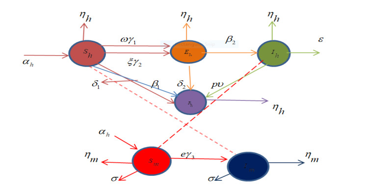
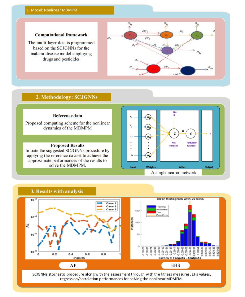
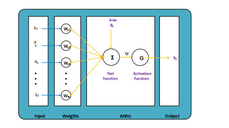
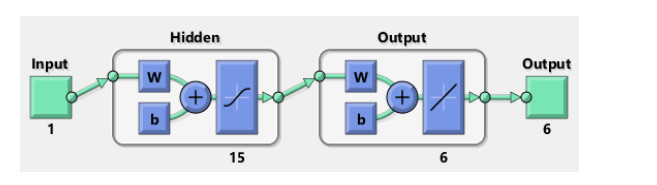
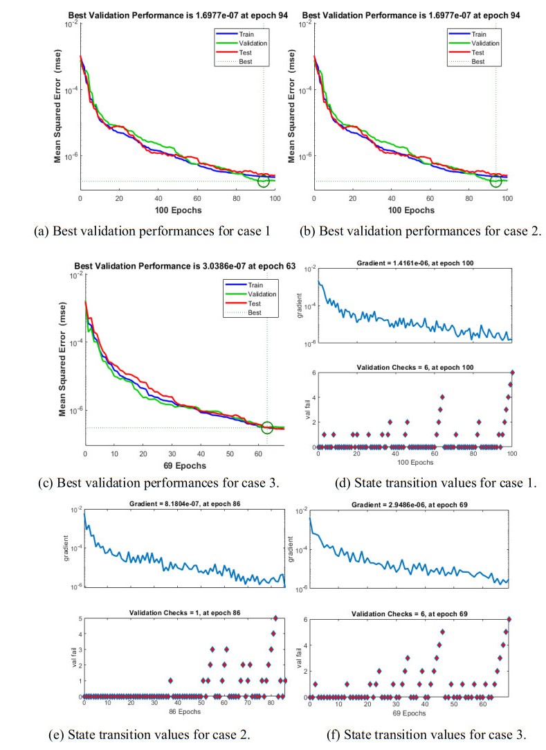
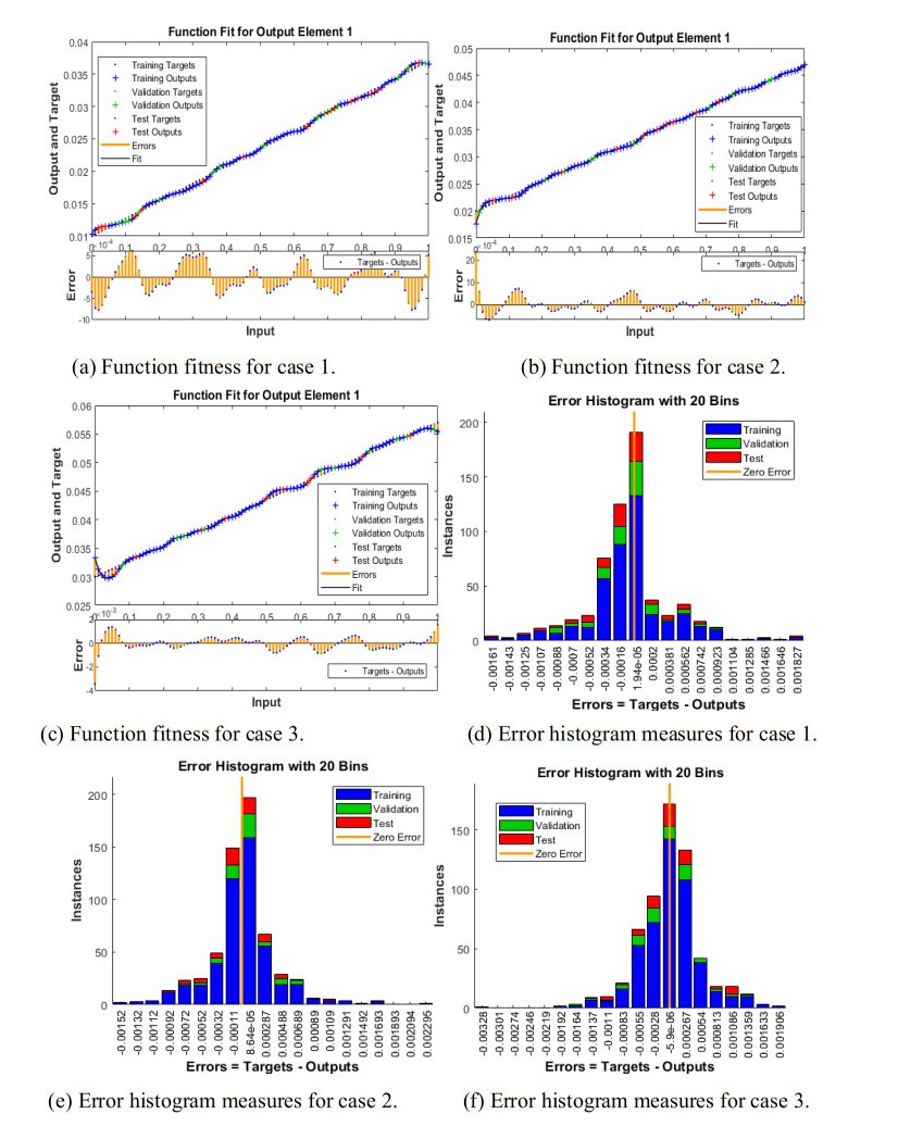
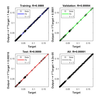
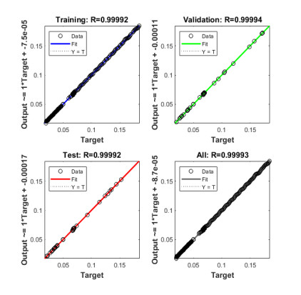
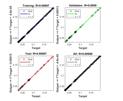
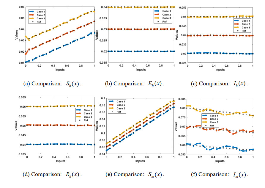
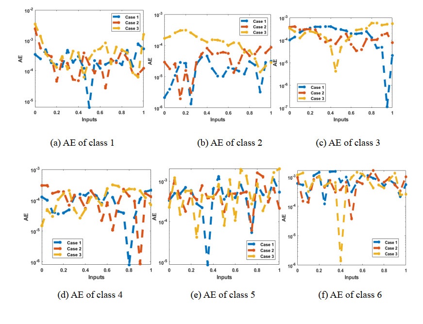
The purpose of this work is to provide a stochastic framework based on the scale conjugate gradient neural networks (SCJGNNs) for solving the malaria disease model of pesticides and medication (MDMPM). The host and vector populations are divided in the mathematical form of the malaria through the pesticides and medication. The stochastic SCJGNNs procedure has been presented through the supervised neural networks based on the statics of validation (12%), testing (10%), and training (78%) for solving the MDMPM. The optimization is performed through the SCJGNN along with the log-sigmoid transfer function in the hidden layers along with fifteen numbers of neurons to solve the MDMPM. The accurateness and precision of the proposed SCJGNNs is observed through the comparison of obtained and source (Runge-Kutta) results, while the small calculated absolute error indicate the exactitude of designed framework based on the SCJGNNs. The reliability and consistency of the SCJGNNs is observed by using the process of correlation, histogram curves, regression, and function fitness.
Citation: Manal Alqhtani, J.F. Gómez-Aguilar, Khaled M. Saad, Zulqurnain Sabir, Eduardo Pérez-Careta. A scale conjugate neural network learning process for the nonlinear malaria disease model[J]. AIMS Mathematics, 2023, 8(9): 21106-21122. doi: 10.3934/math.20231075
The purpose of this work is to provide a stochastic framework based on the scale conjugate gradient neural networks (SCJGNNs) for solving the malaria disease model of pesticides and medication (MDMPM). The host and vector populations are divided in the mathematical form of the malaria through the pesticides and medication. The stochastic SCJGNNs procedure has been presented through the supervised neural networks based on the statics of validation (12%), testing (10%), and training (78%) for solving the MDMPM. The optimization is performed through the SCJGNN along with the log-sigmoid transfer function in the hidden layers along with fifteen numbers of neurons to solve the MDMPM. The accurateness and precision of the proposed SCJGNNs is observed through the comparison of obtained and source (Runge-Kutta) results, while the small calculated absolute error indicate the exactitude of designed framework based on the SCJGNNs. The reliability and consistency of the SCJGNNs is observed by using the process of correlation, histogram curves, regression, and function fitness.

| [1] |
L. Cai, M. Martcheva, X. Z. Li, Epidemic models with age of infection, indirect transmission and incomplete treatment, Discrete Cont. Dyn-B, 18 (2013), 2239. https://doi.org/10.3934/dcdsb.2013.18.2239 doi: 10.3934/dcdsb.2013.18.2239

|
| [2] |
K. W. Blayneh, J. Mohammed-Awel, Insecticide-resistant mosquitoes and malaria control, Math. Biosci., 1 (2014), 252, 14–26. https://doi.org/10.1016/j.mbs.2014.03.007 doi: 10.1016/j.mbs.2014.03.007
|
| [3] | B. A. Johnson, M. G. Kalra, Prevention of malaria in travelers, Am. Fam. Physician, 85 (2012), 973–977. |
| [4] | A. Prabowo, Malaria: Mencegah dan Mengatasi, Niaga Swadaya, 2004. |
| [5] |
B. Breedlove, Public health posters take aim against bloodthirsty ann, Emerg. Infect. Dis., 27 (2021), 676. https://doi.org/10.3201/eid2702.AC2702 doi: 10.3201/eid2702.AC2702
|
| [6] |
L. Basnarkov, I. Tomovski, T. Sandev, L. Kocarev, Non-Markovian SIR epidemic spreading model of COVID-19, Chaos, Soliton. Fract., 1 (2022), 112286. https://doi.org/10.1016/j.chaos.2022.112286 doi: 10.1016/j.chaos.2022.112286
|
| [7] |
M. Sinan, H. Ahmad, Z. Ahmad, J. Baili, S. Murtaza, M. A. Aiyashi, et al., Fractional mathematical modeling of malaria disease with treatment & insecticides, Results Phys., 34 (2022), 105220. https://doi.org/10.1016/j.rinp.2022.105220 doi: 10.1016/j.rinp.2022.105220
|
| [8] |
S. Kumar, A. Ahmadian, R. Kumar, D. Kumar, J. Singh, D. Baleanu, et al., An efficient numerical method for fractional SIR epidemic model of infectious disease by using Bernstein wavelets, Mathematics, 8 (2020), 558. https://doi.org/10.3390/math8040558 doi: 10.3390/math8040558
|
| [9] | F. Haq, K. Shah, A. Khan, M. Shahzad, Numerical solution of fractional order epidemic model of a vector born disease by Laplace Adomian decomposition method, Punjab Univ. J. Math., 49 (2020), 1–8. |
| [10] |
P. Veeresha, E. Ilhan, D. G. Prakasha, H. M. Baskonus, W. Gao, A new numerical investigation of fractional order susceptible-infected-recovered epidemic model of childhood disease, Alex. Eng. J., 61 (2022), 1747–1756. https://doi.org/10.1016/j.aej.2021.07.015 doi: 10.1016/j.aej.2021.07.015
|
| [11] |
P. Veeresha, H. M. Baskonus, D. G. Prakasha, W. Gao, G. Yel, Regarding new numerical solution of fractional Schistosomiasis disease arising in biological phenomena, Chaos, Soliton. Fract., 133 (2020), 109661. https://doi.org/10.1016/j.chaos.2020.109661 doi: 10.1016/j.chaos.2020.109661
|
| [12] |
L.V. Madden, M. J. Jeger, F. Van den Bosch, A theoretical assessment of the effects of vector-virus transmission mechanism on plant virus disease epidemics, Phytopathology, 90 (2000), 576–594. https://doi.org/10.1094/PHYTO.2000.90.6.576 doi: 10.1094/PHYTO.2000.90.6.576
|
| [13] |
A. M. S. Mahdy, M. S. Mohamed, K. Lotfy, M. Alhazmi, A. A. El-Bary, M. H. Raddadi, Numerical solution and dynamical behaviors for solving fractional nonlinear Rubella ailment disease model, Results Phys., 24 (2021), 104091. https://doi.org/10.1016/j.rinp.2021.104091 doi: 10.1016/j.rinp.2021.104091
|
| [14] |
A. Hidalgo, L. Tello, E. F. Toro, Numerical and analytical study of an atherosclerosis inflammatory disease model, J. Math. Biol., 68 (2014), 1785–1814. https://doi.org/10.1007/s00285-013-0688-0 doi: 10.1007/s00285-013-0688-0
|
| [15] |
Y. G. Sánchez, Z. Sabir, J. L. Guirao, Design of a nonlinear SITR fractal model based on the dynamics of a novel coronavirus (COVID-19), Fractals, 28 (2020), 2040026. https://doi.org/10.1142/S0218348X20400265 doi: 10.1142/S0218348X20400265
|
| [16] |
Y. Guerrero Sánchez, Z. Sabir, H. Günerhan, H. M. Baskonus, Analytical and approximate solutions of a novel nervous stomach mathematical model, Discrete Dyn. Nat. Soc., 2020 (2020), 1–13. https://doi.org/10.1155/2020/5063271 doi: 10.1155/2020/5063271
|
| [17] |
K. Cooke, P. Van den Driessche, X. Zou, Interaction of maturation delay and nonlinear birth in population and epidemic models, J. Math. Biol., 39 (1999), 332–352. https://doi.org/10.1007/s002850050194 doi: 10.1007/s002850050194
|
| [18] |
T. Rhodes, Mathematical models as public troubles in COVID-19 infection control: Following the numbers, Health Sociol. Rev., 29 (2020), 177–194. https://doi.org/10.1080/14461242.2020.1764376 doi: 10.1080/14461242.2020.1764376
|
| [19] |
D. Benvenuto, Application of the ARIMA model on the COVID-2019 epidemic dataset, Data Brief, 29 (2020), 105340. https://doi.org/10.1016/j.dib.2020.105340 doi: 10.1016/j.dib.2020.105340
|
| [20] | A. Sivakumar, Review of mathematical models to predict the rate of spread and control of COVID-19 in India, Bull World Health Organ, 2020. |
| [21] | S. K. Mustafa, Brief review of the mathematical models for analyzing and forecasting transmission of COVID-19, 2020. |
| [22] |
R. N. Thompson, Epidemiological models are important tools for guiding COVID-19 interventions, BMC Med., 18 (2020), 1–4. https://doi.org/10.1186/s12916-020-01628-4 doi: 10.1186/s12916-020-01628-4
|
| [23] |
I. Ahmad, M. A. Z. Raja, H. Ramos, M. Bilal, M. Shoaib, Integrated neuro-evolution-based computing solver for dynamics of nonlinear corneal shape model numerically, Neural Comput. Appl., 33 (2021), 5753–5769. https://doi.org/10.1007/s00521-020-05355-y doi: 10.1007/s00521-020-05355-y
|
| [24] |
B. Wang, J. F. Gómez-Aguilar, Z. Sabir, M. A. Z. Raja, W. F. Xia, H. Jahanshahi, et al., Numerical computing to solve the nonlinear corneal system of eye surgery using the capability of Morlet wavelet artificial neural networks, Fractals, 1 (2022), 2240147. https://doi.org/10.1142/S0218348X22401478 doi: 10.1142/S0218348X22401478
|
| [25] |
Z. Sabir, M. A. Z. Raja, S. R. Mahmoud, M. Balubaid, A. Algarni, A. H. Alghtani, et al., A novel design of morlet wavelet to solve the dynamics of nervous stomach nonlinear model, Int. J. Comput. Int. Sys., 15 (2022), 1–4. https://doi.org/10.1007/s44196-021-00057-2 doi: 10.1007/s44196-021-00057-2
|
| [26] |
T. Mouktonglang, Z. Sabir, M. A. Z. Raja, S. Bhatti, T. Botmart, W. Weera, et al., Designing Meyer wavelet neural networks for the three-species food chain model, AIMS Math., 8 (2023), 61–75. https://doi.org/10.3934/math.2023003 doi: 10.3934/math.2023003
|
| [27] |
Z. Sabir, M. A. Z. Raja, A. S. Alnahdi, M. B. Jeelani, M. A. Abdelkawy, Numerical investigations of the nonlinear smoke model using the Gudermannian neural networks, Math. Biosci. Eng., 19 (2022), 351–370. https://doi.org/10.3934/mbe.2022018 doi: 10.3934/mbe.2022018
|
| [28] |
K. Mukdasai, Z. Sabir, M. A. Z. Raja, R. Sadat, M. R. Ali, P. Singkibud, A numerical simulation of the fractional order Leptospirosis model using the supervise neural network, Alex. Eng. J., 61 (2022), 12431–12441. https://doi.org/10.1016/j.aej.2022.06.013 doi: 10.1016/j.aej.2022.06.013
|
| [29] |
T. Botmart, Z. Sabir, M. A. Z. Raja, M. R. Ali, R. Sadat, A. A. Aly, et al., A hybrid swarming computing approach to solve the biological nonlinear Leptospirosis system, Biomed. Signal Proces., 77 (2022), 103789. https://doi.org/10.1016/j.bspc.2022.103789 doi: 10.1016/j.bspc.2022.103789
|
| [30] |
Z. Sabir, Neuron analysis through the swarming procedures for the singular two-point boundary value problems arising in the theory of thermal explosion, Eur. Phys. J. Plus, 137 (2022), 638. https://doi.org/10.1140/epjp/s13360-022-02869-3 doi: 10.1140/epjp/s13360-022-02869-3
|
| [31] |
Z. Sabir, M. A. Manzar, M. A. Z. Raja, M. Sheraz, A. M. Wazwaz, Neuro-heuristics for nonlinear singular Thomas-Fermi systems, Appl. Soft Comput., 65 (2018), 152–169. https://doi.org/10.1016/j.asoc.2018.01.009 doi: 10.1016/j.asoc.2018.01.009
|
| [32] |
H. Liu, T. Liu, Z. Zhang, A. K. Sangaiah, B. Yang, Y. Li, ARHPE: Asymmetric relation-aware representation learning for head pose estimation in industrial human–computer interaction, IEEE T. Ind. Inform., 18 (2022), 7107–7117. https://doi.org/10.1109/TⅡ.2022.3143605 doi: 10.1109/TⅡ.2022.3143605
|
| [33] |
H. Liu, T. Liu, Y. Chen, Z. Zhang, Y. F. Li, EHPE: Skeleton cues-based gaussian coordinate encoding for efficient human pose estimation, IEEE T. Multimedia, 1 (2022), 1–16. https://doi.org/10.1109/TMM.2022.3197364 doi: 10.1109/TMM.2022.3197364
|
| [34] |
H. Liu, S. Fang, Z. Zhang, D. Li, K. Lin, J. Wang, MFDNet: Collaborative poses perception and matrix Fisher distribution for head pose estimation, IEEE T. Multimedia, 24 (2021), 2449–2460. https://doi.org/10.1109/TMM.2021.3081873 doi: 10.1109/TMM.2021.3081873
|
| [35] |
H. Ilyas, I. Ahmad, M. A. Z. Raja, M. Shoaib, A novel design of Gaussian WaveNets for rotational hybrid nanofluidic flow over a stretching sheet involving thermal radiation, Int. Commun. Heat Mass, 123 (2021), 105196. https://doi.org/10.1016/j.icheatmasstransfer.2021.105196 doi: 10.1016/j.icheatmasstransfer.2021.105196
|
| [36] |
M. Dewasurendra, K. Vajravelu, On the method of inverse mapping for solutions of coupled systems of nonlinear differential equations arising in nanofluid flow, heat and mass transfer, Appl. Math. Nonlin. Sci., 3 (2018), 1–14. https://doi.org/10.21042/AMNS.2018.1.00001 doi: 10.21042/AMNS.2018.1.00001
|
| [37] |
A. Yokuş, S. Gülbahar, Numerical solutions with linearization techniques of the fractional Harry Dym equation, Appl. Math. Nonlin. Sci., 4 (2019), 35–42. https://doi.org/10.2478/AMNS.2019.1.00004 doi: 10.2478/AMNS.2019.1.00004
|
| [38] |
H. Rahaman, M. K. Hasan, A. Ali, M. S. Alam, Implicit methods for numerical solution of singular initial value problems, Appl. Math. Nonlin. Sci., 6 (2021), 1–8. https://doi.org/10.2478/amns.2020.2.00001 doi: 10.2478/amns.2020.2.00001
|
| [39] |
A. H. Bukhari, M. A. Z. Raja, N. Rafiq, M. Shoaib, A. K. Kiani, C. M. Shu, Design of intelligent computing networks for nonlinear chaotic fractional Rossler system, Chaos, Soliton. Fract., 157 (2022), 111985. https://doi.org/10.1016/j.chaos.2022.111985 doi: 10.1016/j.chaos.2022.111985
|
| [40] |
X. Li, T. Li, S. Li, B. Tian, J. Ju, T. Liu, et al., Learning fusion feature representation for garbage image classification model in human-robot interaction, Infrared Phys. Techn., 128 (2023), 104457. https://doi.org/10.1016/j.infrared.2022.104457 doi: 10.1016/j.infrared.2022.104457
|
| [41] |
T. Liu, J. Wang, B. Yang, X. Wang, Facial expression recognition method with multi-label distribution learning for non-verbal behavior understanding in the classroom, Infrared Phys. Techn., 112 (2021), 103594. https://doi.org/10.1016/j.infrared.2020.103594 doi: 10.1016/j.infrared.2020.103594
|
| [42] |
T. Liu, J. Wang, B. Yang, X. Wang, NGDNet: Nonuniform Gaussian-label distribution learning for infrared head pose estimation and on-task behavior understanding in the classroom, Neurocomputing, 436 (2021), 210–220. https://doi.org/10.1016/j.neucom.2020.12.090 doi: 10.1016/j.neucom.2020.12.090
|
| [43] |
M. Shoaib, M. A. Z. Raja, M. T. Sabir, A. H. Bukhari, H. Alrabaiah, Z. Shah, et al., A stochastic numerical analysis based on hybrid NAR-RBFs networks nonlinear SITR model for novel COVID-19 dynamics, Comput. Meth. Prog. Bio., 202 (2021), 105973. https://doi.org/10.1016/j.cmpb.2021.105973 doi: 10.1016/j.cmpb.2021.105973
|
Figures(11) / Tables(2)

Manal Alqhtani, J.F. Gómez-Aguilar, Khaled M. Saad, Zulqurnain Sabir, Eduardo Pérez-Careta. A scale conjugate neural network learning process for the nonlinear malaria disease model[J]. AIMS Mathematics, 2023, 8(9): 21106-21122. doi: 10.3934/math.20231075


 DownLoad: