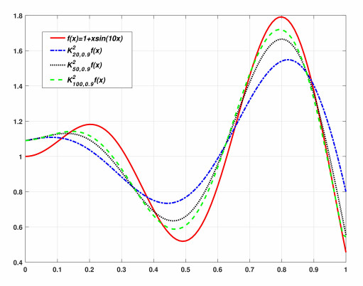
In this paper, we introduce new type of generalized Kantorovich variant of $ \alpha $-Bernstein operators and study their approximation properties. We obtain estimates of rate of convergence involving first and second order modulus of continuity and Lipschitz function are studied for these operators. Furthermore, we establish Voronovskaya type theorem of these operators. The last section is devoted to bivariate new type $ \alpha $-Bernstein-Kantorovich operators and their approximation behaviors. Also, some graphical illustrations and numerical results are provided.
Citation: Mustafa Kara. Approximation properties of the new type generalized Bernstein-Kantorovich operators[J]. AIMS Mathematics, 2022, 7(3): 3826-3844. doi: 10.3934/math.2022212
In this paper, we introduce new type of generalized Kantorovich variant of $ \alpha $-Bernstein operators and study their approximation properties. We obtain estimates of rate of convergence involving first and second order modulus of continuity and Lipschitz function are studied for these operators. Furthermore, we establish Voronovskaya type theorem of these operators. The last section is devoted to bivariate new type $ \alpha $-Bernstein-Kantorovich operators and their approximation behaviors. Also, some graphical illustrations and numerical results are provided.

| [1] |
X. Chen, J. Tan, Z. Liu, J. Xie, Approximation of functions by a new family of generalized Bernstein operator, J. Math. Anal. Appl., 450 (2017), 244–261. doi: 10.1016/j.jmaa.2016.12.075. doi: 10.1016/j.jmaa.2016.12.075

|
| [2] |
S. A. Mohiuddine, T. Acar, A. Alotaibi, Construction of a new family of Bernstein-Kantorovich operators, Math. Method. Appl. Sci., 40 (2017), 7749–7759. doi: 10.1002/mma.4559. doi: 10.1002/mma.4559
|
| [3] | V. I. Volkov, On the convergence of sequences of linear positive operators in the space of continuous functions of two variables, Dokl. Akad. Nauk, 115 (1957), 17–19. |
| [4] | G. G. Lorentz, Bernstein polynomials, Toronto: Univ. of Toronto Press, 1953. |
| [5] | A. Lupas, A q-analogue of the Bernstein operator, University of Cluj-Napoca, Seminar on Numerical and Statistical Calculus, 1987. |
| [6] |
N. Deo, M. Dhamija, Better approximation results by Bernstein-Kantorovich operators, Lobachevskii J. Math., 38 (2017), 94–100. doi: 10.1134/S1995080217010085. doi: 10.1134/S1995080217010085
|
| [7] |
H. Gonska, M. Heilmann, I. Raşa, Kantorovich operators of order k, Numer. Func. Anal. Opt., 32 (2011), 717–738. doi: 10.1080/01630563.2011.580877. doi: 10.1080/01630563.2011.580877
|
| [8] |
M. A. Özarslan, O. Duman, Smoothness poperties of modified Bernstein-Kantorovich operators, Numer. Func. Anal. Opt., 37 (2016), 92–105. doi: 10.1080/01630563.2015.1079219. doi: 10.1080/01630563.2015.1079219
|
| [9] |
N. Mahmudov, P. Sabancıgil, Approximation theorems for $q $-Bernstein-Kantorovich operators, Filomat, 27 (2013), 721–730. doi: 10.2298/FIL1304721M. doi: 10.2298/FIL1304721M
|
| [10] |
T. Acar, A. Aral, S. A. Mohiuddine, On Kantorovich modification of $(p, q)$-Bernstein operators, Iran. J. Sci. Technol. A, 42 (2018), 1459–1464. doi: 10.1007/s40995-017. doi: 10.1007/s40995-017
|
| [11] |
F. Özger, Weighted statistical approximation properties of univariate and bivariate $\lambda $-Kantorovich operators, Filomat, 33 (2019), 3473–3486. doi: 10.2298/FIL1911473O. doi: 10.2298/FIL1911473O
|
| [12] |
T. Acar, A. Aral, S. A. Mohiuddine, Approximation by bivariate $(p, q)$-Bernstein-Kantorovich operators, Iran. J. Sci. Technol. A, 4 (2018), 655–662. doi: 10.1007/s40995-016-0045-4. doi: 10.1007/s40995-016-0045-4
|
| [13] | T. Acar, A. Aral, S. A. Mohiuddine, On Kantorovich modification of ($p, q)$-Baskakov operators, J. Inequal. Appl., 98 (2016). doi: 10.1186/s13660-016-1045-9. |
| [14] |
A. M. Acu, C. Muraru, Approximation properties of bivariate extension of $q$-Bernstein-Schurer Kantorovich operators, Results Math., 67 (2015), 265–279. doi: 10.1007/s00025-015-0441-7. doi: 10.1007/s00025-015-0441-7
|
| [15] | Q. B. Cai, The Bézier variant of Kantorovich type $\lambda $-Bernstein operators, J. Inequal. Appl., 90 (2018). doi: 10.1186/s13660-018-1688-9. |
| [16] |
S. A. Mohiuddine, T. Acar, A. Alotaibi, Construction of a new family of Bernstein-Kantorovich operators, Math. Method. Appl. Sci., 40 (2017), 7749–7759. doi: 10.1002/mma.4559. doi: 10.1002/mma.4559
|
| [17] |
N. Deo, R. Pratap, $\alpha $-Bernstein-Kantorovich operators, Afr. Mat., 31 (2020), 609–618. doi: 10.1007/s13370-019-00746-4. doi: 10.1007/s13370-019-00746-4
|
| [18] | S. A. Mohiuddine, F. Özger, Approximation of functions by Stancu variant of Bernstein-Kantorovich operators based on shape parameter, RACSAM Rev. R. Acad. A, 70 (2020). doi: 10.1007/s13398-020-00802-w. |
| [19] |
Q. B. Cai, W. T. Cheng, B. Çekim, Bivariate $\alpha, q$ -Bernstein-Kantorovich operators and GBS operators of Bivariate $\alpha, q$ -Bernstein-Kantorovich type, Mathematics, 7 (2019), 1161. doi: 10.3390/math7121161. doi: 10.3390/math7121161
|
| [20] |
A. Kajla, P. Agarwal, S. Araci, A Kantorovich variant of a generalized Bernstein operators, J. Math. Comput. Sci., 19 (2019), 86–96. doi: 10.22436/jmcs.019.02.03. doi: 10.22436/jmcs.019.02.03
|
| [21] | R. A. Devore, G. G. Lorentz, Constructive approximation, Springer-Verlang, New York, 1993. |
| [22] |
M. A. Özarslan, H. Aktuğlu, Local Approximation peroperties for certain King type operators, Filomat, 27 (2013), 173–182. doi: 10.2298/FILI301173Oç. doi: 10.2298/FILI301173Oç
|
| [23] | Z. Ditzion, V. Totik, Moduli of smoothness, Springer-Verlag, New York, 1987. doi: 10.1007/978-1-4612-4778-7. |


Figures(3) / Tables(1)

Mustafa Kara. Approximation properties of the new type generalized Bernstein-Kantorovich operators[J]. AIMS Mathematics, 2022, 7(3): 3826-3844. doi: 10.3934/math.2022212


 DownLoad: