Plenty of wave solutions to the ill-posed Boussinesq dynamic wave equation under shallow water beneath gravity

Mostafa M. A. Khater; S. H. Alfalqi; J. F. Alzaidi; Samir A. Salama; Fuzhang Wang; Mostafa M. A. Khater; S. H. Alfalqi; J. F. Alzaidi; Samir A. Salama; Fuzhang Wang

doi:10.3934/math.2022004

AIMS Mathematics

2022, Volume 7, Issue 1: 54-81. doi: 10.3934/math.2022004

Previous Article Next Article

Research article

Plenty of wave solutions to the ill-posed Boussinesq dynamic wave equation under shallow water beneath gravity

1.
Department of Mathematics, Faculty of Science, Jiangsu University, 212013 Zhenjiang, China
2.
Department of Mathematics, Obour High Institute For Engineering and Technology, 11828 Cairo, Egypt
3.
Department of Mathematics, Faculty of Science and Arts, Mahayil Asir King Khalid University, Abha, Saudi Arabia
4.
Division of Biochemistry, Department of Pharmacology, College of Pharmacy, Taif University, P.O. Box 11099, Taif 21944, Saudi Arabia
5.
School of Mathematical and Statistics, Xuzhou University of Technology, Xuzhou 221018, Jiangsu, China
6.
Nanchang Institute of Technology, Nanchang 330044, China
7.
College of Computer Science and Technology, Huaibei Normal University, 235000 Huaibei, China

Received: 27 June 2021 Accepted: 16 August 2021 Published: 29 September 2021
MSC : 35C08, 34A25, 49M05

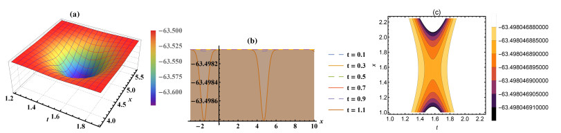
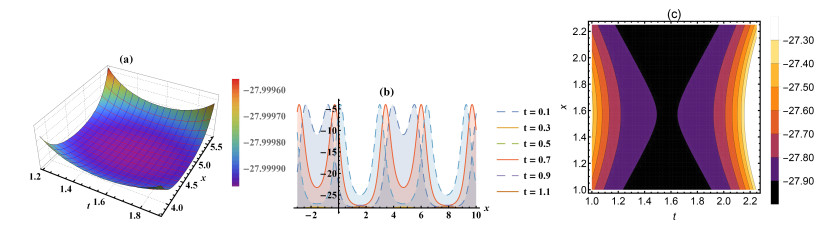
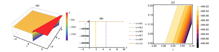
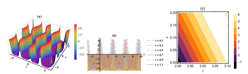
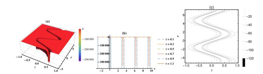
This paper applies two computational techniques for constructing novel solitary wave solutions of the ill-posed Boussinesq dynamic wave (IPB) equation. Jacques Hadamard has formulated this model for studying the dynamic behavior of waves in shallow water under gravity. Extended simple equation (ESE) method and novel Riccati expansion (NRE) method have been applied to the investigated model's converted nonlinear ordinary differential equation through the wave transformation. As a result of this research, many solitary wave solutions have been obtained and represented in different figures in two-dimensional, three-dimensional, and density plots. The explanation of the methods used shows their dynamics and effectiveness in dealing with certain nonlinear evolution equations.
Citation: Mostafa M. A. Khater, S. H. Alfalqi, J. F. Alzaidi, Samir A. Salama, Fuzhang Wang. Plenty of wave solutions to the ill-posed Boussinesq dynamic wave equation under shallow water beneath gravity[J]. AIMS Mathematics, 2022, 7(1): 54-81. doi: 10.3934/math.2022004

Related Papers:

Abstract

This paper applies two computational techniques for constructing novel solitary wave solutions of the ill-posed Boussinesq dynamic wave (IPB) equation. Jacques Hadamard has formulated this model for studying the dynamic behavior of waves in shallow water under gravity. Extended simple equation (ESE) method and novel Riccati expansion (NRE) method have been applied to the investigated model's converted nonlinear ordinary differential equation through the wave transformation. As a result of this research, many solitary wave solutions have been obtained and represented in different figures in two-dimensional, three-dimensional, and density plots. The explanation of the methods used shows their dynamics and effectiveness in dealing with certain nonlinear evolution equations.

References

[1]	D. D. Holm, J. E. Marsden, T. S. Ratiu, The euler-Poincaré equations and semidirect products with applications to continuum theories, Adv. Math., 137 (1998), 1–81. doi: 10.1006/aima.1998.1721. doi: 10.1006/aima.1998.1721
[2]	V. I. Sbitnev, Bohmian trajectories and the path integral paradigm: Complexified lagrangian mechanics, Int. J. Bifurcat. Chaos, 19 (2009), 2335–2346. doi: 10.1142/S0218127409024104. doi: 10.1142/S0218127409024104
[3]	M. M. Khater, M. Inc, K. Nisar, R. A. Attia, Multi-solitons, lumps, and breath solutions of the water wave propagation with surface tension via four recent computational schemes, Ain Shams Eng. J., 12 (2021), 3031–3041. doi: 10.1016/j.asej.2020.10.029. doi: 10.1016/j.asej.2020.10.029
[4]	M. M. Khater, M. S. Mohamed, R. A. Attia, On semi analytical and numerical simulations for a mathematical biological model; the time-fractional nonlinear Kolmogorov-Petrovskii-Piskunov (KPP) equation, Chaos Soliton. Fract., 144 (2021), 110676. doi: 10.1016/j.chaos.2021.110676. doi: 10.1016/j.chaos.2021.110676
[5]	M. M. Khater, A. Mousa, M. El-Shorbagy, R. A. Attia, Analytical and semi-analytical solutions for Phi-four equation through three recent schemes, Results Phys., 2021, 103954. doi: 10.1016/j.rinp.2021.103954.
[6]	M. M. Khater, A. E. S. Ahmed, M. El-Shorbagy, Abundant stable computational solutions of Atangana-Baleanu fractional nonlinear HIV-1 infection of CD4+ T-cells of immunodeficiency syndrome, Results Phys., 144 (2021), 103890. doi: 10.1016/j.rinp.2021.103890. doi: 10.1016/j.rinp.2021.103890
[7]	M. M. Khater, S. Anwar, K. U. Tariq, M. S. Mohamed, Some optical soliton solutions to the perturbed nonlinear Schrödinger equation by modified Khater method, AIP Adv., 11 (2021), 025130. doi: 10.1063/5.0038671. doi: 10.1063/5.0038671
[8]	M. M. Khater, R. A. Attia, A. Bekir, D. Lu, Optical soliton structure of the sub-10-fs-pulse propagation model, J. Opt., 50 (2021), 109–119. doi: 10.1007/s12596-020-00667-7. doi: 10.1007/s12596-020-00667-7
[9]	Y. Chu, M. M. Khater, Y. Hamed, Diverse novel analytical and semi-analytical wave solutions of the generalized (2+1)-dimensional shallow water waves model, AIP Adv., 11 (2021), 015223. doi: 10.1063/5.0036261. doi: 10.1063/5.0036261
[10]	R. A. Attia, D. Baleanu, D. Lu, M. M. Khater, E. S. Ahmed, Computational and numerical simulations for the deoxyribonucleic acid (DNA) model, Discrete Cont. Dyn-S., 14 (2021), 3459–3478. doi: 10.3934/dcdss.2021018. doi: 10.3934/dcdss.2021018
[11]	M. M. Khater, A. Bekir, D. Lu, R. A. Attia, Analytical and semi-analytical solutions for time-fractional Cahn-Allen equation, Math. Method. Appl. Sci., 44 (2021), 2682–2691. doi: 10.1002/mma.6951. doi: 10.1002/mma.6951
[12]	A. Saha, K. K. Ali, H. Rezazadeh, Y. Ghatani, Analytical optical pulses and bifurcation analysis for the traveling optical pulses of the hyperbolic nonlinear Schrödinger equation, Opt. Quant. Electron., 53 (2021), 1–19. doi: 10.1007/s11082-021-02787-1. doi: 10.1007/s11082-021-02787-1
[13]	H. Rezazadeh, M. Odabasi, K. U. Tariq, R. Abazari, H. M. Baskonus, On the conformable nonlinear Schrödinger equation with second order spatiotemporal and group velocity dispersion coefficients, Chinese J. Phys., 72 (2021), 403–414. doi: 10.1016/j.cjph.2021.01.012. doi: 10.1016/j.cjph.2021.01.012
[14]	F. Tchier, A. I. Aliyu, A. Yusuf, Dynamics of solitons to the ill-posed Boussinesq equation, Eur. Phys. J. Plus, 132 (2017), 1–9. doi: 10.1140/epjp/i2017-11430-0. doi: 10.1140/epjp/i2017-11430-0
[15]	S. Duran, M. Askin, T. A. Sulaiman, New soliton properties to the ill-posed Boussinesq equation arising in nonlinear physical science, Int. J. Opt. Control (IJOCTA), 7 (2017), 240–247. doi: 10.11121/ijocta.01.2017.00495. doi: 10.11121/ijocta.01.2017.00495
[16]	P. Daripa, W. Hua, A numerical study of an ill-posed Boussinesq equation arising in water waves and nonlinear lattices: Filtering and regularization techniques, Appl. Math. Comput., 101 (1999), 159–207. doi; 10.1016/S0096-3003(98)10070-X.
[17]	S. Bibi, N. Ahmed, U. Khan, S. T. Mohyud-Din, Auxiliary equation method for ill-posed Boussinesq equation, Phys. Scripta, 94 (2019), 085213. doi: 10.1088/1402-4896/ab1951. doi: 10.1088/1402-4896/ab1951
[18]	C. Park, M. M. Khater, A. H. Abdel-Aty, R. A. Attia, H. Rezazadeh, A. Zidan, et al., Dynamical analysis of the nonlinear complex fractional emerging telecommunication model with higher-order dispersive cubic-quintic, Alex. Eng. J., 59 (2020), 1425–1433. doi: 10.1016/j.aej.2020.03.046. doi: 10.1016/j.aej.2020.03.046
[19]	M. M. Khater, R. A. Attia, A. H. Abdel-Aty, W. Alharbi, D. Lu, Abundant analytical and numerical solutions of the fractional microbiological densities model in bacteria cell as a result of diffusion mechanisms, Chaos Soliton. Fract., 136 (2020), 109824. doi: 10.1016/j.chaos.2020.109824. doi: 10.1016/j.chaos.2020.109824
[20]	C. Park, M. M. Khater, A. H. Abdel-Aty, R. A. Attia, D. Lu, On new computational and numerical solutions of the modified Zakharov-Kuznetsov equation arising in electrical engineering, Alex. Eng. J., 59 (2020), 1099–1105. doi: 10.1016/j.aej.2019.12.043. doi: 10.1016/j.aej.2019.12.043
[21]	M. M. Khater, R. A. Attia, A. H. Abdel-Aty, M. Abdou, H. Eleuch, D. Lu, Analytical and semi-analytical ample solutions of the higher-order nonlinear Schrödinger equation with the non-kerr nonlinear term, Results Phys., 16 (2020), 103000. doi: 10.1016/j.rinp.2020.103000. doi: 10.1016/j.rinp.2020.103000
[22]	D. Lu, M. Osman, M. M. Khater, R. A. Attia, D. Baleanu, Analytical and numerical simulations for the kinetics of phase separation in iron (Fe–Cr–X (X = Mo, Cu)) based on ternary alloys, Physica A, 537 (2020), 122634. doi: 10.1016/j.physa.2019.122634. doi: 10.1016/j.physa.2019.122634
[23]	A. T. Ali, M. M. Khater, R. A. Attia, A. H. Abdel-Aty, D. Lu, Abundant numerical and analytical solutions of the generalized formula of Hirota-Satsuma coupled KdV system, Chaos Soliton. Fract., 131 (2020), 109473. doi: 10.1016/j.chaos.2019.109473. doi: 10.1016/j.chaos.2019.109473
[24]	A. H. Abdel-Aty, M. M. Khater, H. Dutta, J. Bouslimi, M. Omri, Computational solutions of the HIV-1 infection of CD4$^{+}$ T-cells fractional mathematical model that causes acquired immunodeficiency syndrome (AIDS) with the effect of antiviral drug therapy, Chaos Soliton. Fract., 139 (2020), 110092. doi: 10.1016/j.chaos.2020.110092. doi: 10.1016/j.chaos.2020.110092
[25]	B. Gao, H. Tian, Symmetry reductions and exact solutions to the ill-posed Boussinesq equation, Int. J. Nonlin. Mech., 72 (2015), 80–83. doi: 10.1016/j.ijnonlinmec.2015.03.004. doi: 10.1016/j.ijnonlinmec.2015.03.004
[26]	F. Wang, H. Cheng, J. Si, Response solution to ill-posed Boussinesq equation with quasi-periodic forcing of Liouvillean frequency, J. Nonlinear Sci., 30 (2021), 657–710. doi: 10.1007/s00332-019-09587-8. doi: 10.1007/s00332-019-09587-8
[27]	E. Yaşar, S. San, Y. S. Özkan, Nonlinear self adjointness, conservation laws and exact solutions of ill-posed Boussinesq equation, Open Phys., 14 (2016), 37–43. doi: 10.1515/phys-2016-0007. doi: 10.1515/phys-2016-0007
[28]	N. Kishimoto, Sharp local well-posedness for the "good" Boussinesq equation, J. Differ. Equations, 254 (2013), 2393–2433. doi: 10.1016/j.jde.2012.12.008. doi: 10.1016/j.jde.2012.12.008
[29]	R. Temam, J. Tribbia, Open boundary conditions for the primitive and Boussinesq equations, J. Atmos. Sci., 60 (2003), 2647–2660. doi: 10.1175/1520-0469(2003)060<2647:obcftp>2.0.co;2. doi: 10.1175/1520-0469(2003)060<2647:obcftp>2.0.co;2
[30]	H. Cheng, R. de la Llave, Stable manifolds to bounded solutions in possibly ill-posed PDEs, J. Differ. Equations, 268 (2020), 4830–4899. doi: 10.1016/j.jde.2019.10.042. doi: 10.1016/j.jde.2019.10.042

Reader Comments

Your name:*

Email:*
© 2022 the Author(s), licensee AIMS Press. This is an open access article distributed under the terms of the Creative Commons Attribution License (http://creativecommons.org/licenses/by/4.0)