Study of wind speed and relative humidity using stochastic technique in a semi-arid climate region

Suhail Mahmud; Md Al Masum Bhuiyan; Nusrat Sarmin; Sanjida Elahee; Suhail Mahmud; Md Al Masum Bhuiyan; Nusrat Sarmin; Sanjida Elahee

doi:10.3934/environsci.2020010

AIMS Environmental Science

2020, Volume 7, Issue 2: 156-173. doi: 10.3934/environsci.2020010

Previous Article Next Article

Research article

Study of wind speed and relative humidity using stochastic technique in a semi-arid climate region

1.
Department of Computational Science, University of Texas at El Paso, 500 w university avenue, El Paso, TX 79912, USA
2.
Department of Computer Science, University of Texas at El Paso, 500 w university avenue, El Paso, TX 79912, USA
3.
Department of Chemistry, University of Delaware, Newark, DE 19716, USA

Received: 19 September 2019 Accepted: 21 February 2020 Published: 24 March 2020

This paper deals with the stochastic analysis of wind speed based on relative humidity data. We propose a stochastic regression technique to estimate the time-varying parameters of wind speed in a semi-arid climate region. The modeling of stochastic parameters of atmospheric data with consistent properties facilitates prediction with higher precision. In order to compare the estimation, we used simulated atmospheric time series and observational time series. The atmospheric time series was generated by the Weather Research and Forecasting (WRF) model, whereas the observational time series was obtained from the surface weather stations. The time-varying parameters of the model used are estimated by Maximum Likelihood process. The results obtained suggest that relative humidity exhibits a stochastic effect to predict stationary wind speed data. This type of analysis helps to characterize some key meteorological variables, which would be useful in forecasting irregular wind speed.
- wind speed,
- relative humidity,
- maximum likelihood estimation,
- stochastic regression,
- bootstrapping,
- WRF model
Citation: Suhail Mahmud, Md Al Masum Bhuiyan, Nusrat Sarmin, Sanjida Elahee. Study of wind speed and relative humidity using stochastic technique in a semi-arid climate region[J]. AIMS Environmental Science, 2020, 7(2): 156-173. doi: 10.3934/environsci.2020010

Related Papers:

Abstract

This paper deals with the stochastic analysis of wind speed based on relative humidity data. We propose a stochastic regression technique to estimate the time-varying parameters of wind speed in a semi-arid climate region. The modeling of stochastic parameters of atmospheric data with consistent properties facilitates prediction with higher precision. In order to compare the estimation, we used simulated atmospheric time series and observational time series. The atmospheric time series was generated by the Weather Research and Forecasting (WRF) model, whereas the observational time series was obtained from the surface weather stations. The time-varying parameters of the model used are estimated by Maximum Likelihood process. The results obtained suggest that relative humidity exhibits a stochastic effect to predict stationary wind speed data. This type of analysis helps to characterize some key meteorological variables, which would be useful in forecasting irregular wind speed.

References

[1]	Kavasseri RG, Seetharaman K (2009) Day-ahead wind speed forecasting using f-ARIMA models. Renew Energ 34: 1388-1393. doi: 10.1016/j.renene.2008.09.006
[2]	Cassola F, Burlando M (2012) Wind speed and wind energy forecast through Kalman filtering of Numerical Weather Prediction model output. Appl Energ 99: 154-166. doi: 10.1016/j.apenergy.2012.03.054
[3]	Warner TT, Peterson RA, Treadon RE (1997) A tutorial on lateral boundary conditions as a basic and potentially serious limitation to regional numerical weather prediction. B Am Meteorol Soc 78: 2599-2618. doi: 10.1175/1520-0477(1997)078<2599:ATOLBC>2.0.CO;2
[4]	Franzke CL, O'Kane TJ, Berner J, et al. (2015) Stochastic climate theory and modeling. Wiley Interdis Rev: Climate Change 6: 63-78. doi: 10.1002/wcc.318
[5]	Yu Media Group. El Paso, TX. Detailed climate information and monthly weather forecast. Available from https://www.weather-us.com/en/texas-usa/el-paso-climate.
[6]	Misachi J (2017) What Are The Characteristics Of A Semi-arid Climate Pattern. Available from: https://www.worldatlas.com/articles/what-are-the-characteristics-of-a-semi-arid-climate pattern.html
[7]	Novlan DJ, Hardiman M, Gill TE (2007) A synoptic climatology of blowing dust events in El Paso, Texas from 1932-2005. In Preprints, 16th Conference on Applied Climatology, American Meteorological Society J
[8]	Breshears DD, Kirchner TB, Whicker JJ, et al. (2012) Modeling aeolian transport in response to succession, disturbance and future climate: Dynamic long-term risk assessment for contaminant redistribution. Aeolian Res 3: 445-457. doi: 10.1016/j.aeolia.2011.03.012
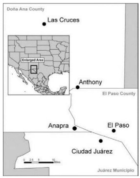
[9]	Regional Stakeholders Committee (2009) The Paso Del Norte Region, US-Mexico: Self-Evaluation Report, OECD Reviews of Higher Education in Regional and City Development, IMHE. Available from: https://www.oecd.org/unitedstates/44210876.pdf
[10]	Baumbach JP, Foster LN, Mueller M, et al. (2008) Seroprevalence of select blood borne pathogens and associated risk behaviors among injection drug users in the Paso del Norte region of the United States-Mexico border. Harm Reduct J 5: 33. doi: 10.1186/1477-7517-5-33
[11]	Lu D, Reddy R, Fitzgerald R, et al. (2008) Sensitivity modeling study for an ozone occurrence during the 1996 Paso del Norte ozone campaign. Int J Environ Res Pub He 5: 181-203. doi: 10.3390/ijerph5040181
[12]	Pearson R, Fitzgerald R (2005) Application of a wind model for the El Paso-Juarez airshed. J Air Waste Manage Assoc 51: 669-680.
[13]	Cai C, Kelly JT, Avise Stockwell WR, et al. (2001) Photochemical modeling in California with two chemical mechanisms: model intercomparison and response to emission reductions. J Air Waste Manage Assoc 61: 559-572.
[14]	Mahmud S, Wangchuk P, Fitzgerald R, et al. (2016) Study of Photolysis Rate Coefficients to Improve Air Quality Models. B Am Phy Soc 61.
[15]	Mahmud S (2016) The use of remote sensing technologies and models to study pollutants in the Paso del Norte region. The University of Texas at El Paso. Available from: https://scholarworks.utep.edu/open_etd/685/
[16]	Ullwer C, Sprung D, Sucher E, et al. (2019) Global simulations of Cn2 using the Weather Research and Forecast Model WRF and comparison to experimental results. In Laser communication and Propagation through the Atmosphere and Oceans VIII: 111330I
[17]	Brown MJ, Muller C, Wang W (2001) Costigan, K. Meteorological simulations of boundary layer structure during the 1996 Paso del Norte Ozone Study. Sci Total Environ. 276: 111-133.
[18]	Michalakes J, Dudhia J, Gill D, et al. (2005) The weather research and forecast model: software architecture and performance. Use High Perform Comput Meteorol 2005: 156-168.
[19]	Michalakes J, Chen S, Dudhia J, et al. (2001) Development of a next-generation regional weather research and forecast model. Dev Teracomput 2001: 269-276.
[20]	Skamarock WC, Klemp J B, Dudhia J, et al. (2005) A description of the advanced research WRF version 2 (No. NCAR/TN-468+ STR). National Center for Atmospheric Research Boulder Co Mesoscale and Microscale Meteorology Div.
[21]	Islam MR, Peace A, Medina D, Oraby T (2020) Integer versus Fractional Order SEIR Deterministic and Stochastic Models of Measles. Int J Env Res Pub He 17: 2014. doi: 10.3390/ijerph17062014
[22]	Allen DT, Torres VM (2010) TCEQ Flare Study Project, Final Report. The University of Texas at Austin The Center for Energy and Environmental Resources.
[23]	Wilby RL, Charles SP, Zorita E, et al. (2004) Guidelines for use of climate scenarios developed from statistical downscaling methods. Supporting material of the Intergovernmental Panel on Climate Change, available from the DDC of IPCC TGCIA 27.
[24]	Raysoni AU, Sarnat JA, Sarnat SE, et al. (2011) Binational school-based monitoring of traffic-related air pollutants in El Paso, Texas (USA) and Ciudad Jurez, Chihuahua (Mxico). Env Pol 159: 2476-2486. doi: 10.1016/j.envpol.2011.06.024
[25]	Said SE, Dickey D (1984) Testing for Unit Roots in Autoregressive Moving-Average Models with Unknown Order. Biometrika 71: 599-607. doi: 10.1093/biomet/71.3.599
[26]	Phillips PCB, Perron Pierre (1988) Testing for a Unit Root in Time Series Regression. Biometrika 75: 335-346. doi: 10.1093/biomet/75.2.335
[27]	Wellner Jon A (2003) Gaussian White Noise Models: Some Results for Monotone Functions. Lecture Notes-Monograph Series 2003: 87-104.
[28]	Kitagawa G (1994) State Space Modeling of Time Series. The Institute of Statistical Mathematics 43-64.
[29]	Grineski SE, Collins TW, McDonald YJ, et al. (2015) Double exposure and the climate gap: changing demographics and extreme heat in Ciudad Jurez, Mexico. Local Env 20: 180-201. doi: 10.1080/13549839.2013.839644
[30]	Wilder M, Garfin G, Ganster P, et al. (2013) Climate change and US-Mexico border communities. In Assessment of Climate Change in the Southwest United States, Island Press, Washington DC: 340-384.

Reader Comments

your name:*

Email:*
© 2020 the Author(s), licensee AIMS Press. This is an open access article distributed under the terms of the Creative Commons Attribution License (http://creativecommons.org/licenses/by/4.0)