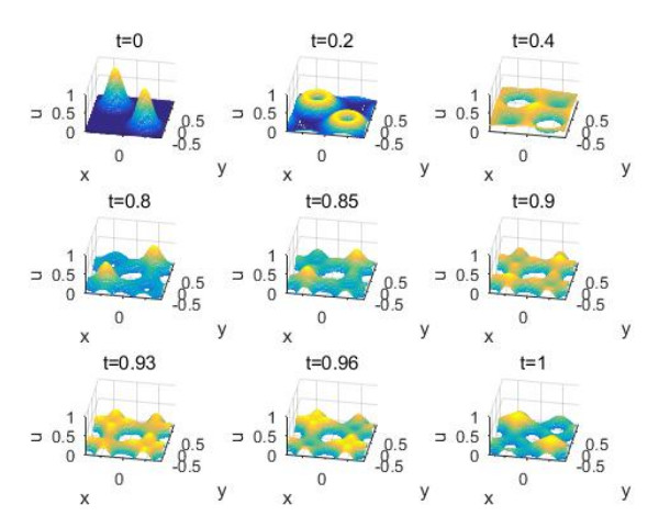
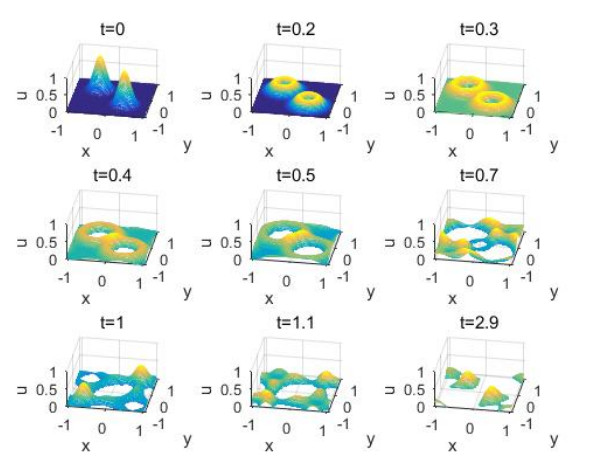
This paper is mainly concerned with the initial boundary value problems of semilinear wave equations with damping term and mass term as well as Neumann boundary conditions on exterior domain in three dimensions. Blow-up and upper bound lifespan estimates of solutions to the problem with damping term and mass term are derived by applying test function technique and iterative method, where nonlinear terms are power nonlinearity $ |u|^p $, derivative nonlinearity $ |u_{t}|^p $, combined nonlinearities $ |u_t|^p+|u|^q $, respectively. Moreover, upper bound lifespan estimate of solution to the problem with scale invariant damping term, non-negative mass term and combined nonlinearities $ |u_t|^p+|u|^q $ is obtained. The proofs are based on the test function method and iterative approach. The main new contribution is that upper bound lifespan estimates of solutions are associated with the Strauss exponent and Glassey exponent. In addition, the variation trend of wave is achieved by taking advantage of numerical simulation.
Citation: Xiongmei Fan, Sen Ming, Wei Han, Zikun Liang. Lifespan estimate of solution to the semilinear wave equation with damping term and mass term[J]. AIMS Mathematics, 2023, 8(8): 17860-17889. doi: 10.3934/math.2023910
This paper is mainly concerned with the initial boundary value problems of semilinear wave equations with damping term and mass term as well as Neumann boundary conditions on exterior domain in three dimensions. Blow-up and upper bound lifespan estimates of solutions to the problem with damping term and mass term are derived by applying test function technique and iterative method, where nonlinear terms are power nonlinearity $ |u|^p $, derivative nonlinearity $ |u_{t}|^p $, combined nonlinearities $ |u_t|^p+|u|^q $, respectively. Moreover, upper bound lifespan estimate of solution to the problem with scale invariant damping term, non-negative mass term and combined nonlinearities $ |u_t|^p+|u|^q $ is obtained. The proofs are based on the test function method and iterative approach. The main new contribution is that upper bound lifespan estimates of solutions are associated with the Strauss exponent and Glassey exponent. In addition, the variation trend of wave is achieved by taking advantage of numerical simulation.

| [1] |
W. H. Chen, T. A. Dao, On the Cauchy problem for semilinear regularity-loss-type $\sigma$-evolution models with memory term, Nonlinear Anal. Real World Appl., 59 (2021), 103265. https://doi.org/10.1016/j.nonrwa.2020.103265 doi: 10.1016/j.nonrwa.2020.103265

|
| [2] |
W. H. Chen, T. A. Dao, Sharp lifespan estimates for the weakly coupled system of semilinear damped wave equations in the critical case, Math. Ann., 385 (2023), 101–130. https://doi.org/10.1007/s00208-021-02335-y doi: 10.1007/s00208-021-02335-y
|
| [3] |
Y. X. Chen, R. Z. Xu, Global well-posedness of solutions for fourth order dispersive wave equation with nonlinear weak damping, linear strong damping and logarithmic nonlinearity, Nonlinear Anal., 192 (2020), 111664. https://doi.org/10.1016/j.na.2019.111664 doi: 10.1016/j.na.2019.111664
|
| [4] |
F. A. Chiarello, G. Girardi, S. Lucente, Fujita modified exponent for scale invariant damped semilinear wave equation, arXiv, 2020. https://doi.org/10.48550/arXiv.2002.03418 doi: 10.48550/arXiv.2002.03418
|
| [5] |
W. Dai, H. Kubo, M. Sobajima, Blow-up for Strauss type wave equation with damping and potential, Nonlinear Anal.: Real World Appl., 57 (2021), 103195. https://doi.org/10.1016/j.nonrwa.2020.103195 doi: 10.1016/j.nonrwa.2020.103195
|
| [6] |
T. A. Dao, A result for non-existence of global solutions to semilinear structural damped wave model, arXiv, 2019. https://doi.org/10.48550/arXiv.1912.07066 doi: 10.48550/arXiv.1912.07066
|
| [7] |
T. A. Dao, A. Z. Fino, Critical exponent for semilinear structurally damped wave equation of derivative type, Math. Methods Appl. Sci., 43 (2020), 9766–9775. https://doi.org/10.1002/mma.6649. doi: 10.1002/mma.6649
|
| [8] |
F. Q. Du, J. H. Hao, Energy decay for wave equation of variable coefficients with dynamic boundary conditions and time varying delay, J. Geom. Anal., 33 (2023), 119. https://doi.org/10.1007/s12220-022-01161-1 doi: 10.1007/s12220-022-01161-1
|
| [9] |
V. Georgiev, A. Palmieri, Critical exponent of Fujita type for the semilinear damped wave equation on the Heisenberg group with power nonlinearity, J. Differ. Equations, 269 (2020), 420–448. https://doi.org/10.1016/j.jde.2019.12.009 doi: 10.1016/j.jde.2019.12.009
|
| [10] |
V. Georgiev, A. Palmieri, Lifespan estimates for local in time solutions to the semilinear heat equation on the Heisenberg group, Ann. Mat. Pura Appl., 200 (2021), 999–1032. https://doi.org/10.1007/s10231-020-01023-z doi: 10.1007/s10231-020-01023-z
|
| [11] |
M. Hamouda, M. A. Hamza, A blow-up result for the wave equation with localized initial data: the scale invariant damping and mass term with combined nonlinearities, arXiv, 2020. https://doi.org/10.48550/arXiv.2010.05455 doi: 10.48550/arXiv.2010.05455
|
| [12] |
M. Hamouda, M. A. Hamaz, Blow-up for wave equation with the scale invariant damping and combined nonlinearities, Math. Methods Appl. Sci., 44 (2021), 1127–1136. https://doi.org/10.1002/mma.6817 doi: 10.1002/mma.6817
|
| [13] |
W. Han, Y. Zhou, Blow-up for some semilinear wave equations in multi-space dimensions, Commun. Partial Differ. Equ., 39 (2014), 651–665. https://doi.org/10.1080/03605302.2013.863916 doi: 10.1080/03605302.2013.863916
|
| [14] |
K. Hidano, C. B. Wang, K. Yokoyama, Combined effects of two nonlinearities in lifespan of small solutions to semilinear wave equations, Math. Ann., 366 (2016), 667–694. https://doi.org/10.1007/s00208-015-1346-1 doi: 10.1007/s00208-015-1346-1
|
| [15] |
M. Ikeda, M. Sobajima, K. Wakasa, Blow-up phenomena of semilinear wave equations and their weakly coupled systems, J. Differ. Equations, 267 (2019), 5165–5201. https://doi.org/10.1016/j.jde.2019.05.029 doi: 10.1016/j.jde.2019.05.029
|
| [16] |
M. Ikeda, T. Tanaka, K. Wakasa, Critical exponent for the wave equation with a time dependent scale invariant damping and a cubic convolution, J. Differ. Equations, 270 (2021), 916–946. https://doi.org/10.1016/j.jde.2020.08.047 doi: 10.1016/j.jde.2020.08.047
|
| [17] |
M. Ikeda, Z. H. Tu, K. Wakasa, Small data blow-up of semilinear wave equation with scattering dissipation and time dependent mass, Evol. Equ. Control The., 11 (2021), 515–536. https://doi.org/10.3934/eect.2021011 doi: 10.3934/eect.2021011
|
| [18] |
T. Imai, M. Kato, H. Takamura, K. Wakasa, The lifespan of solutions of semilinear wave equations with the scale invariant damping in two space dimensions, J. Differ. Equations, 269 (2020), 8387–8424. https://doi.org/10.1016/j.jde.2020.06.019 doi: 10.1016/j.jde.2020.06.019
|
| [19] |
F. John, Blow-up for quasilinear wave equations in three space dimensions, Commun. Pure Appl. Math., 34 (1981), 29–51. https://doi.org/10.1002/cpa.3160340103 doi: 10.1002/cpa.3160340103
|
| [20] |
S. Kitamura, K. Morisawa, H. Takamura, The lifespan of classical solutions of semilinear wave equations with spatial weights and compactly supported data in one space dimension, J. Differ. Equations, 307 (2022), 486–516. https://doi.org/10.1016/j.jde.2021.10.062 doi: 10.1016/j.jde.2021.10.062
|
| [21] |
N. A. Lai, M. Y. Liu, Z. H. Tu, C. B. Wang, Lifespan estimates for semilinear wave equations with space dependent damping and potential, Calc. Var. Partial Differ. Equ., 62 (2023), 44. https://doi.org/10.1007/s00526-022-02388-0 doi: 10.1007/s00526-022-02388-0
|
| [22] | N. A. Lai, N. M. Schiavone, H. Takamura, Wave-like blow-up for semilinear wave equations with scattering damping and negative mass term, In: M. D'Abbicco, M. Ebert, V. Georgiev, T. Ozawa, New tools for nonlinear PDEs and application, Trends in Mathematics, Birkhäuser, Cham, 2019,217–240. https://doi.org/10.1007/978-3-030-10937-0_8 |
| [23] |
N. A. Lai, N. M. Schiavone, H. Takamura, Heat like and wave like lifespan estimates for solutions of semilinear damped wave equations via a Kato's type lemma, J. Differ. Equations, 269 (2020), 11575–11620. https://doi.org/10.1016/j.jde.2020.08.020 doi: 10.1016/j.jde.2020.08.020
|
| [24] |
N. A. Lai, H. Takamura, Blow-up for semilinear damped wave equations with sub-critical exponent in the scattering case, Nonlinear Anal., 168 (2018), 222–237. https://doi.org/10.1016/J.NA.2017.12.008 doi: 10.1016/J.NA.2017.12.008
|
| [25] |
N. A. Lai, H. Takamura, Non-existence of global solutions of nonlinear wave equations with weak time dependent damping related to Glassey's conjecture, Differ. Integr. Equ., 32 (2019), 37–48. https://doi.org/10.57262/die/1544497285 doi: 10.57262/die/1544497285
|
| [26] |
N. A. Lai, H. Takamura, Non-existence of global solutions of wave equations with weak time dependent damping and combined nonlinearity, Nonlinear Anal.: Real World Appl., 45 (2019), 83–96. https://doi.org/10.1016/j.nonrwa.2018.06.008 doi: 10.1016/j.nonrwa.2018.06.008
|
| [27] |
N. A. Lai, H. Takamura, K. Wakasa, Blow-up for semilinear wave equations with the scale invariant damping and super Fujita exponent, J. Differ. Equations, 263 (2017), 5377–5394. https://doi.org/10.1016/j.jde.2017.06.017 doi: 10.1016/j.jde.2017.06.017
|
| [28] |
N. A. Lai, Z. H. Tu, Strauss exponent for semilinear wave equations with scattering space dependent damping, J. Math. Anal. Appl., 489 (2020), 124189. https://doi.org/10.1016/j.jmaa.2020.124189 doi: 10.1016/j.jmaa.2020.124189
|
| [29] |
N. A. Lai, Y. Zhou, Blow-up and lifespan estimate to a nonlinear wave equation in Schwarzschild spacetime, J. Math. Pures Appl., 173 (2023), 172–194. https://doi.org/10.1016/j.matpur.2023.02.009 doi: 10.1016/j.matpur.2023.02.009
|
| [30] |
Q. Lei, H. Yang, Global existence and blow-up for semilinear wave equations with variable coefficients, Chin. Ann. Math. Ser. B, 39 (2018), 643–664. https://doi.org/10.1007/s11401-018-0087-3 doi: 10.1007/s11401-018-0087-3
|
| [31] |
Y. H. Lin, N. A. Lai, S. Ming, Lifespan estimate for semilinear wave equation in Schwarzschild spacetime, Appl. Math. Lett., 99 (2020), 105997. https://doi.org/10.1016/j.aml.2019.105997 doi: 10.1016/j.aml.2019.105997
|
| [32] |
M. Y. Liu, C. B. Wang, Blow-up for small amplitude semilinear wave equations with mixed nonlinearities on asymptotically Euclidean manifolds, J. Differ. Equations, 269 (2020), 8573–8596. https://doi.org/10.1016/j.jde.2020.06.032 doi: 10.1016/j.jde.2020.06.032
|
| [33] |
S. Ming, S. Y. Lai, X. M. Fan, Lifespan estimates of solutions to quasilinear wave equations with scattering damping, J. Math. Anal. Appl., 492 (2020), 124441. https://doi.org/10.1016/j.jmaa.2020.124441 doi: 10.1016/j.jmaa.2020.124441
|
| [34] |
S. Ming, S. Y. Lai, X. M. Fan, Blow-up for a coupled system of semilinear wave equations with scattering dampings and combined nonlinearities, Appl. Anal., 101 (2022), 2996–3016. https://doi.org/10.1080/00036811.2020.1834086 doi: 10.1080/00036811.2020.1834086
|
| [35] |
A. Palmieri, H. Takamura, Blow-up for a weakly coupled system of semilinear damped wave equations in the scattering case with power nonlinearities, Nonlinear Anal., 187 (2019), 467–492. https://doi.org/10.1016/j.na.2019.06.016 doi: 10.1016/j.na.2019.06.016
|
| [36] |
A. Palmieri, Z. H. Tu, Lifespan of semilinear wave equation with scale invariant dissipation and mass and sub-Strauss power nonlinearity, J. Math. Anal. Appl., 470 (2019), 447–469. https://doi.org/10.1016/j.jmaa.2018.10.015 doi: 10.1016/j.jmaa.2018.10.015
|
| [37] |
A. Palmieri, Z. H. Tu, A blow-up result for a semilinear wave equation with scale invariant damping and mass and nonlinearity of derivative type, Calc. Var. Partial Differ. Equ., 60 (2021), 72. https://doi.org/10.1007/s00526-021-01948-0 doi: 10.1007/s00526-021-01948-0
|
| [38] |
K. Wakasa, B. Yordanov, On the non-existence of global solutions for critical semilinear wave equations with damping in the scattering case, Nonlinear Anal., 180 (2019), 67–74. https://doi.org/10.1016/j.na.2018.09.012 doi: 10.1016/j.na.2018.09.012
|
| [39] |
K. Wakasa, B. Yordanov, Blow-up of solutions to critical semilinear wave equations with variable coefficients, J. Differ. Equations, 266 (2019), 5360–5376. https://doi.org/10.1016/j.jde.2018.10.028 doi: 10.1016/j.jde.2018.10.028
|
| [40] |
Y. Zhou, Blow up of solutions to semilinear wave equations with critical exponent in high dimensions, Chin. Ann. Math. Ser. B, 28 (2007), 205–212. https://doi.org/10.1007/s11401-005-0205-x doi: 10.1007/s11401-005-0205-x
|
| [41] |
Y. Zhou, W. Han, Blow-up of solutions to semilinear wave equations with variable coefficients and boundary, J. Math. Anal. Appl., 374 (2011), 585–601. https://doi.org/10.1016/j.jmaa.2010.08.052 doi: 10.1016/j.jmaa.2010.08.052
|
| [42] |
Y. Zhou, W. Han, Lifespan of solutions to critical semilinear wave equations, Commun. Partial Differ. Equ., 39 (2014), 439–451. https://doi.org/10.1080/03605302.2013.863914 doi: 10.1080/03605302.2013.863914
|
Figures(2)

Xiongmei Fan, Sen Ming, Wei Han, Zikun Liang. Lifespan estimate of solution to the semilinear wave equation with damping term and mass term[J]. AIMS Mathematics, 2023, 8(8): 17860-17889. doi: 10.3934/math.2023910


 DownLoad: