The finite time blow-up for Caputo-Hadamard fractional diffusion equation involving nonlinear memory

Zhiqiang Li; Zhiqiang Li

doi:10.3934/math.2022715

AIMS Mathematics

2022, Volume 7, Issue 7: 12913-12934. doi: 10.3934/math.2022715

Previous Article Next Article

Research article

The finite time blow-up for Caputo-Hadamard fractional diffusion equation involving nonlinear memory

Zhiqiang Li ^,

Department of Mathematics, Luliang University, Lvliang, Shanxi 033001, China

Received: 10 March 2022 Revised: 19 April 2022 Accepted: 20 April 2022 Published: 06 May 2022
MSC : 26A33, 35R11, 35B44

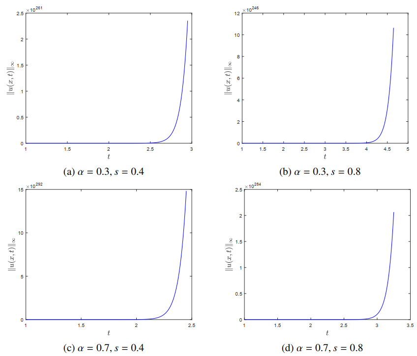
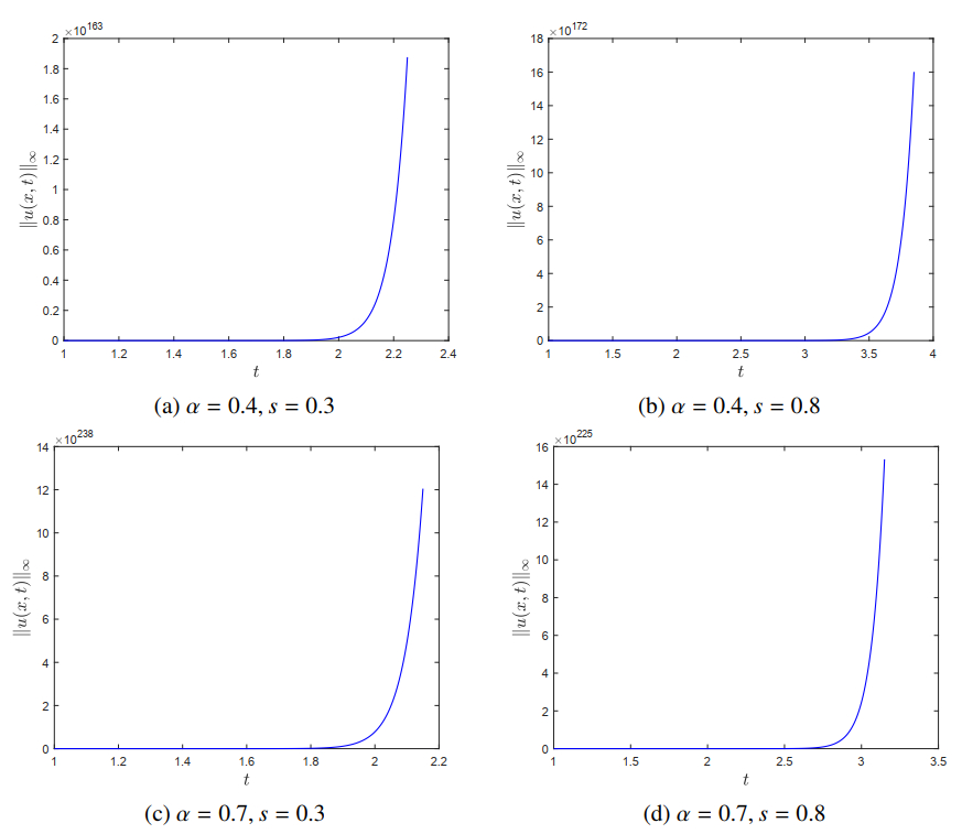
In this article, we focus on the blow-up problem of solution to Caputo-Hadamard fractional diffusion equation with fractional Laplacian and nonlinear memory. By virtue of the fundamental solutions of the corresponding linear and nonhomogeneous equation, we introduce a mild solution of the given equation and prove the existence and uniqueness of local solution. Next, the concept of a weak solution is presented by the test function and the mild solution is demonstrated to be a weak solution. Finally, based on the contraction mapping principle, the finite time blow-up and global solution for the considered equation are shown and the Fujita critical exponent is determined. The finite time blow-up of solution is also confirmed by the results of numerical experiment.
- Caputo-Hadamard derivative,
- fractional Laplacian,
- nonlinear memory,
- finite time blow-up,
- fixed point argument
Citation: Zhiqiang Li. The finite time blow-up for Caputo-Hadamard fractional diffusion equation involving nonlinear memory[J]. AIMS Mathematics, 2022, 7(7): 12913-12934. doi: 10.3934/math.2022715

Related Papers:

Abstract

In this article, we focus on the blow-up problem of solution to Caputo-Hadamard fractional diffusion equation with fractional Laplacian and nonlinear memory. By virtue of the fundamental solutions of the corresponding linear and nonhomogeneous equation, we introduce a mild solution of the given equation and prove the existence and uniqueness of local solution. Next, the concept of a weak solution is presented by the test function and the mild solution is demonstrated to be a weak solution. Finally, based on the contraction mapping principle, the finite time blow-up and global solution for the considered equation are shown and the Fujita critical exponent is determined. The finite time blow-up of solution is also confirmed by the results of numerical experiment.

References

[1]	K. B. Oldham, J. Spanier, The fractional calculus, New York: Academic Press, 1974.
[2]	S. G. Samko, A. A. Kilbas, O. I. Marichev, Fractional integrals and derivatives: Theory and applications, Amsterdam: Gordon and Breach Science, 1993.
[3]	I. Podlubny, Fractional differential equations, New York: Academic Press, 1999.
[4]	A. A. Kilbas, H. M. Srivastava, J. J. Trujillo, Theory and applications of fractional differential equations, Amsterdam: Elsevier, 2006.
[5]	Y. G. Sinai, The limiting behavior of a one-dimensional random walk in a random medium, Theor. Probab. Appl., 27 (1983), 256–268. https://doi.org/10.1007/978-1-4419-6205-8 doi: 10.1007/978-1-4419-6205-8
[6]	H. Schiessel, I. M. Sokolov, A. Blumen, Dynamics of a polyampholyte hooked around an obstacle, Phys. Rev. E, 56 (1997), R2390–R2393. https://doi.org/10.1103/PhysRevE.56.R2390 doi: 10.1103/PhysRevE.56.R2390
[7]	S. I. Denisov, H. Kantz, Continuous-time random walk theory of superslow diffusion, Europhys Lett., 92 (2010), 30001. https://doi.org/10.1209/0295-5075/92/30001 doi: 10.1209/0295-5075/92/30001
[8]	W. T. Ang, Hypersingular integral equations in fracture analysis, Amsterdam: Elsevier, 2014.
[9]	R. Garra, F. Mainardi, G. Spada, A generalization of the Lomnitz logarithmic creep law via Hadamard fractional calculus, Chaos Soliton. Fract., 102 (2017), 333–338. https://doi.org/10.1016/j.chaos.2017.03.032 doi: 10.1016/j.chaos.2017.03.032
[10]	Y. Liang, S. Wang, W. Chen, Z. Zhou, R. L. Magin, A survey of models of ultraslow diffusion in heterogeneous materials, Appl. Mech. Rev., 71 (2019), 040802. https://doi.org/10.1115/1.4044055 doi: 10.1115/1.4044055
[11]	A. De Gregorio, R. Garra, Hadamard-type fractional heat equations and ultra-slow diffusions, Fractal Fract., 5 (2021), 48. https://doi.org/10.3390/fractalfract5020048 doi: 10.3390/fractalfract5020048
[12]	J. Hadamard, Essai sur létude des fonctions données par leur développement de Taylor, J. Math. Pures Appl., 8 (1892), 101–186.
[13]	A. A. Kilbas, Hadamard-type fractional calculus, J. Korean Math. Soc., 38 (2001), 1191–1204.
[14]	C. P. Li, Z. Q. Li, Asymptotic behaviors of solution to Caputo-Hadamard fractional partial differential equation with fractional Laplacian, Int. J. Comput. Math., 98 (2021), 305–339.
[15]	C. P. Li, Z. Q. Li, Asymptotic behaviors of solution to partial differential equation with Caputo-Hadamard derivative and fractional Laplacian: Hyperbolic case, Discrete Cont. Dyn.-S., 14 (2021), 3659–3683. https://doi.org/10.3934/dcdss.2021023 doi: 10.3934/dcdss.2021023
[16]	C. P. Li, Z. Q. Li, The blow-up and global existence of solution to Caputo-Hadamard fractional partial differential equation with fractional Laplacian, J. Nonlinear Sci., 31 (2021), 80. https://doi.org/10.1007/s00332-021-09736-y doi: 10.1007/s00332-021-09736-y
[17]	C. P. Li, Z. Q. Li, Stability and logarithmic decay of the solution to Hadamard-type fractional differential equation, J. Nonlinear Sci., 31 (2021), 31. https://doi.org/10.1007/s00332-021-096918 doi: 10.1007/s00332-021-096918
[18]	L. Ma, Blow-up phenomena profile for Hadamard fractional differential systems in finite time, Fractals, 27 (2019), 1950093. https://doi.org/10.1142/S0218348X19500932 doi: 10.1142/S0218348X19500932
[19]	L. Ma, Comparative analysis on the blow-up occurrence of solutions to Hadamard type fractional differential systems, Int. J. Comput. Math., 99 (2022), 895–908. https://doi.org/10.1080/00207160.2021.1939020 doi: 10.1080/00207160.2021.1939020
[20]	E. Di Nezza, G. Palatucci, E. Valdinoci, Hitchhiker's guide to the fractional Sobolev spaces, Bull. Sci. Math., 136 (2011), 521–573. https://doi.org/10.1016/j.bulsci.2011.12.004 doi: 10.1016/j.bulsci.2011.12.004
[21]	C. Bucur, E. Valdinoci, Non-local diffusion and applications, Cham: Springer, 2016.
[22]	X. Ros-Oton, Nonlocal elliptic equations in bounded domains: A survey, Publ. Mat., 60 (2016), 3–26. https://doi.org/10.5565/PUBLMAT_60116_01 doi: 10.5565/PUBLMAT_60116_01
[23]	M. Kwaśnicki, Ten equivalent definitions of the fractional Laplace operator, Frac. Calc. Appl. Anal., 20 (2017), 7–51. https://doi.org/10.1515/fca-2017-0002 doi: 10.1515/fca-2017-0002
[24]	H. Fujita, On the blowing up of solutions of the Cauchy problem for $u_{t} = \Delta u+u^{1+\alpha}$, J. Fac. Sci. Univ. Tokyo Sect. I, 13 (1966), 109–124.
[25]	F. B. Weissler, Existence and nonexistence of global solutions for a semilinear heat equation, Israel J. Math., 38 (1981), 29–40.
[26]	T. Cazenave, F. Dickstein, F. B. Weissler, An equation whose Fujita critical exponent is not given by scaling, Nonlinear Anal., 68 (2008), 862–874. https://doi.org/10.1016/j.na.2006.11.042 doi: 10.1016/j.na.2006.11.042
[27]	P. Souplet, Blow-up in nonlocal reaction-diffusion equations, SIAM J. Math. Anal., 29 (1998), 1301–1334. https://doi.org/10.1137/S0036141097318900 doi: 10.1137/S0036141097318900
[28]	A. Z. Fino, M. Kirane, Qualitative properties of solutions to a time-space fractional evolution equation, Quart. Appl. Math., 70 (2012), 133–157. https://doi.org/10.1090/S0033-569X-2011-01246-9 doi: 10.1090/S0033-569X-2011-01246-9
[29]	Y. N. Li, Q. G. Zhang, Blow-up and global existence of solutions for a time fractional diffusion equation, Frac. Calc. Appl. Anal., 21 (2018), 1619–1640. https://doi.org/10.1515/fca-2018-0085 doi: 10.1515/fca-2018-0085
[30]	C. P. Li, M. Cai, Theory and numerical approximations of fractional integrals and derivatives, Philadelphia: SIAM, 2019.
[31]	F. Jarad, T. Abdeljawad, D. Baleanu, Caputo-type modification of the Hadamard fractional derivatives, Adv. Differ. Equ., 2012 (2012), 142. https://doi.org/10.1186/1687-1847-2012-142 doi: 10.1186/1687-1847-2012-142
[32]	A. A. Kilbas, M. Saigo, $H$-transforms: Theory and applications, Boca Raton: CRC Press, 2004.
[33]	H. M. Srivastava, K. C. Gupta, S. P. Goyal, The $H$-functions of one and two variables with applications, New Delhi: South Asian, 1982.
[34]	Q. G. Zhang, Y. N. Li, The critical exponent for a time fractional diffusion equation with nonlinear memory, Math. Meth. Appl. Sci., 41 (2018), 6443–6456. https://doi.org/10.1002/mma.5169 doi: 10.1002/mma.5169
[35]	M. Gohar, C. P. Li, Z. Q. Li, Finite difference methods for Caputo-Hadamard fractional differential equations, Mediterr. J. Math., 17 (2020), 194. https://doi.org/10.1007/s00009-020-01605-4 doi: 10.1007/s00009-020-01605-4
[36]	S. W. Duo, H. W. V. Wyk, Y. Z. Zhang, A novel and accurate finite difference method for the fractional Laplacian and the fractional Poisson problem, J. Comput. Phys., 355 (2018), 233–252. https://doi.org/10.1016/j.jcp.2017.11.011 doi: 10.1016/j.jcp.2017.11.011

Reader Comments

Your name:*

Email:*
© 2022 the Author(s), licensee AIMS Press. This is an open access article distributed under the terms of the Creative Commons Attribution License (http://creativecommons.org/licenses/by/4.0)