Multi-omics analysis and validation of the tumor microenvironment of hepatocellular carcinoma under RNA modification patterns

Yuanqian Yao; Jianlin Lv; Guangyao Wang; Xiaohua Hong; Yuanqian Yao; Jianlin Lv; Guangyao Wang; Xiaohua Hong

doi:10.3934/mbe.2023814

Mathematical Biosciences and Engineering

2023, Volume 20, Issue 10: 18318-18344. doi: 10.3934/mbe.2023814

Previous Article Next Article

Research article Special Issues

Multi-omics analysis and validation of the tumor microenvironment of hepatocellular carcinoma under RNA modification patterns

1.
Guangxi University of Chinese medicine, NanNing 530000, China
2.
The First Affiliated Hospital of Guangxi University of Chinese Medicine, Nanning 530000, China

Received: 03 July 2023 Revised: 12 August 2023 Accepted: 23 August 2023 Published: 22 September 2023

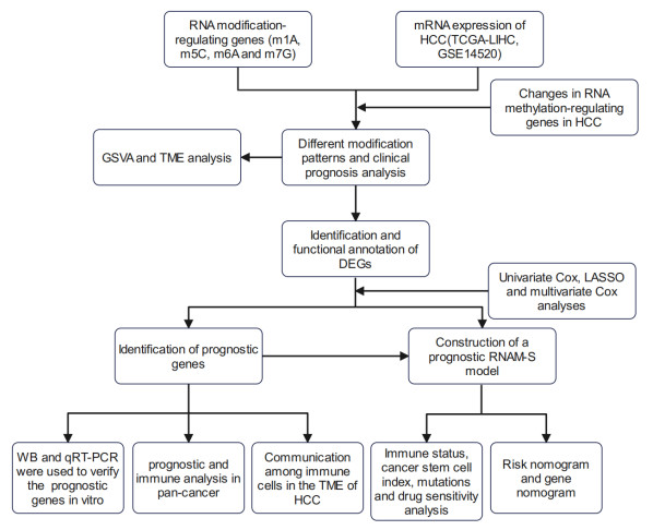
Background: Multiple types of RNA modifications are associated with the prognosis of hepatocellular carcinoma (HCC) patients. However, the overall mediating effect of RNA modifications on the tumor microenvironment (TME) and the prognosis of patients with HCC is unclear. Methods: Thoroughly analyze the TME, biological processes, immune infiltration and patient prognosis based on RNA modification patterns and gene patterns. Construct a prognostic model (RNA modification score, RNAM-S) to predict the overall survival (OS) in HCC patients. Analyze the immune status, cancer stem cell (CSC), mutations and drug sensitivity of HCC patients in both the high and low RNAM-S groups. Verify the expression levels of the four characteristic genes of the prognostic RNAM-S using in vitro cell experiments. Results: Two modification patterns and two gene patterns were identified in this study. Both the high-expression modification pattern and the gene pattern exhibited worse OS. A prognostic RNAM-S model was constructed based on four featured genes (KIF20A, NR1I2, NR2F1 and PLOD2). Cellular experiments suggested significant dysregulation of the expression levels of these four genes. In addition, validation of the RNAM-S model using each data set showed good predictive performance of the model. The two groups of HCC patients (high and low RNAM-S groups) exhibited significant differences in immune status, CSC, mutation and drug sensitivity. Conclusion: The findings of the study demonstrate the clinical value of RNA modifications, which provide new insights into the individualized treatment for patients with HCC.

Keywords:

Citation: Yuanqian Yao, Jianlin Lv, Guangyao Wang, Xiaohua Hong. Multi-omics analysis and validation of the tumor microenvironment of hepatocellular carcinoma under RNA modification patterns[J]. Mathematical Biosciences and Engineering, 2023, 20(10): 18318-18344. doi: 10.3934/mbe.2023814

Related Papers:

[1]	Zhongdi Cen, Jian Huang, Aimin Xu . A posteriori mesh method for a system of singularly perturbed initial value problems. AIMS Mathematics, 2022, 7(9): 16719-16732. doi: 10.3934/math.2022917
[2]	Lin Fan, Shunchu Li, Dongfeng Shao, Xueqian Fu, Pan Liu, Qinmin Gui . Elastic transformation method for solving the initial value problem of variable coefficient nonlinear ordinary differential equations. AIMS Mathematics, 2022, 7(7): 11972-11991. doi: 10.3934/math.2022667
[3]	Shuqin Zhang, Jie Wang, Lei Hu . On definition of solution of initial value problem for fractional differential equation of variable order. AIMS Mathematics, 2021, 6(7): 6845-6867. doi: 10.3934/math.2021401
[4]	Jean-Paul Chehab, Denys Dutykh . On time relaxed schemes and formulations for dispersive wave equations. AIMS Mathematics, 2019, 4(2): 254-278. doi: 10.3934/math.2019.2.254
[5]	Yu He, Jianing Yang, Theodore E. Simos, Charalampos Tsitouras . A novel class of Runge-Kutta-Nyström pairs sharing orders 8(6). AIMS Mathematics, 2024, 9(2): 4882-4895. doi: 10.3934/math.2024237
[6]	Jiadong Qiu, Danfu Han, Hao Zhou . A general conservative eighth-order compact finite difference scheme for the coupled Schrödinger-KdV equations. AIMS Mathematics, 2023, 8(5): 10596-10618. doi: 10.3934/math.2023538
[7]	Sara S. Alzaid, Pawan Kumar Shaw, Sunil Kumar . A numerical study of fractional population growth and nuclear decay model. AIMS Mathematics, 2022, 7(6): 11417-11442. doi: 10.3934/math.2022637
[8]	Daniel Clemente-López, Esteban Tlelo-Cuautle, Luis-Gerardo de la Fraga, José de Jesús Rangel-Magdaleno, Jesus Manuel Munoz-Pacheco . Poincaré maps for detecting chaos in fractional-order systems with hidden attractors for its Kaplan-Yorke dimension optimization. AIMS Mathematics, 2022, 7(4): 5871-5894. doi: 10.3934/math.2022326
[9]	Sen Ming, Xiaodong Wang, Xiongmei Fan, Xiao Wu . Blow-up of solutions for coupled wave equations with damping terms and derivative nonlinearities. AIMS Mathematics, 2024, 9(10): 26854-26876. doi: 10.3934/math.20241307
[10]	Huichol Choi, Kinam Sin, Sunae Pak, Kyongjin Sok, Sungryol So . Representation of solution of initial value problem for fuzzy linear multi-term fractional differential equation with continuous variable coefficient. AIMS Mathematics, 2019, 4(3): 613-625. doi: 10.3934/math.2019.3.613

Abstract

1. Introduction

We are exploring the initial value problem (IVP) defined as:

$\begin{equation} z^{\prime \prime } = f(t,z),\;z(t_{0}) = z_0,\;z^{\prime}(t_0) = z^{\prime}_0, \end{equation}$

(1.1)

where $f: \mathbb{R} \times \mathbb{R}^m\longrightarrow\mathbb{R}^m$ and $z_0, \; z^{\prime}_0\in \mathbb{R}^m$ . The above equation is widely applicable in various scientific and engineering contexts. Notably, Eq (1.1) lacks $z^{\prime }$ .

The Numerov method facilitates the numerical advancement of the solution from $t_k$ to $t_{k+1} = h+t_k$ , a well-established approach for solving Eq (1.1). It is expressed as:

$z_{k+1} = 2z_k-z_{k-1}+\frac{h^2}{12}\left(f_{k+1}+10f_k+f_{k-1}\right),$

where $z_k\approx z(t_k)$ and $f_k\approx z^{\prime \prime }_n = f(t_k, z_k)$ . Note that $f_k, z_k\in\mathbb{R}^m$ .

Hairer ^[1], Cash ^[2] and Chawla ^[3] introduced hybrid implicit Numerov-type methods (i.e., using non-mesh points) approximately 40–45 years ago. Addressing the P-stability property, crucial for handling stiff oscillatory problems, was the primary challenge then. Chawla ^[4] proposed the modified Numerov scheme, evaluated explicitly as follows:

$\begin{equation} \begin{array}{c} v_1 = z_{k-1}, \\ v_2 = z_k, \\ v_3 = 2z_k-z_{k-1}+h^2f(t_k,v_2), \\ z_{k+1}-2z_k+z_{k-1} = \frac{1}{12}h^2\cdot (f(t_{k+1},v_3)+10f(t_k,v_2)+f(t_{k-1},v_1)), \\ \end{array} \end{equation}$

(1.2)

where $h$ is a constant step length:

$h = t_{k}-t_{k-1} = t_{k+1}-t_{k} = \cdots = t_1-t_0.$

The vectors $z_{k+1}, \; z_k$ , and $z_{k-1}$ approximate $z(t_k+h), \; z(t_k)$ , and $z(t_k-h)$ respectively, while $v_1\in\mathbb{R}^m, \; v_2\in\mathbb{R}^m$ , and $v_3\in\mathbb{R}^m$ represent the stages (alternatively named: function evaluations) used by the method.

We utilize the information known at the mesh:

$v_1 = z_{k-1},\:v_2 = z_k.$

Since $f(t_{k-1}, v_1)$ is computed in the previous step, only $f(t_{k+1}, v_3)$ and $f(t_{k}, v_2)$ need evaluation each step, resulting in only two function evaluations per step.

Tsitouras then introduced a Runge–Kutta–Nyström (RKN)-style method ^[5], significantly reducing the cost. Consequently, only four steps are required to create a sixth-order method, whereas previous implementations required six function evaluations (see ^[6]).

Subsequent to this, our group extensively investigated the topic. Tsitouras developed eighth-order methods with nine steps per step in ^[7]. Ninth-order methods were studied in ^[8]. Concurrently, a group of Spanish researchers conducted highly interesting work on the same topic ^[9,10,11].

In this study, we aim to present a new method for better addressing problems with periodic solutions. Traditionally, various properties from a simple test equation are fulfilled for this purpose. The novelty lies in training the available free parameters across a wide set of relevant problems. Differential evolution is employed for this training. It is anticipated that this methodology will yield a method better tuned for oscillatory problems.

2. Order conditions for hybrid Numerov-type methods

For the numerical treatment of Eq (1.1) with higher-order algebraic methods, there exists a considerable demand. We can represent the independent variable $t$ as one of the components of $z$ (if necessary, add $t^{\prime\prime} = 0$ see [, pg. 286] for details). Consequently, our focus, without loss of generality, lies on the autonomous system $z^{\prime\prime} = f(z)$ . Subsequently, a hybrid Numerov method with $s$ stages, as delineated in ^[7], may be expressed as:

$\begin{equation} \begin{array}{c} z_{k+1} = 2z_{k}-z_{k-1}+h^2\cdot \left( w\otimes I_{s}\right) \cdot f\left( v\right) ,\,\ v = \left( \textbf{1}+a\right) \otimes z_{k}-a\otimes z_{k-1}+ h^2\cdot \left( D\otimes I_{s}\right) \cdot f\left( v\right) \end{array} \end{equation}$

(2.1)

where $I_s \in \mathbb{R}^{s \times s}$ represents the identity matrix, $D \in \mathbb{R}^{s\times s}, w^T \in \mathbb{R}^s, a\; \in \mathbb{R}^s$ denote the coefficient matrices of the method, and

$\textbf{1} = [1\; 1\; \cdots 1]^T \in \mathbb{R}^s.$

To present the coefficients, we utilize the Butcher tableau ^[13,14],

$\begin{array}{c|c} a & D \\ \hline & w \end{array}.$

The method described in (1.2) can be represented using matrices ^[8]. As the function evaluations are computed sequentially, these methods are explicit. Therefore, $D$ represents a strictly lower triangular matrix. For the case when $s = 8$ , the method takes the following structure:

$\begin{eqnarray*} f_{k-1} & = &f\left( t_{k-1},z_{k-1}\right) \\ f_{k} & = &f\left( t_{k},z_{k}\right) \\ z_{\alpha} & = &a_{3}z_{k-1}+\left( 1-a_{3}\right) z_{k}+h^{2}\left(d_{31}f_{k-1}+a_{d2}f_{k}\right) ,\ \\ f_{\alpha} & = &f\left( t_{k}-a_{3}h,z_{\alpha}\right) , \\ z_{\beta} & = &a_{4}z_{k-1}+\left( 1-a_{4}\right) z_{k}+h^{2}\left(d_{41}f_{k-1}+d_{42}f_{k}+d_{43}f_{\alpha}\right) , \\ f_{\beta} & = &f\left( t_{k}-a_{4}h,z_{\beta}\right) , \\ z_{c} & = &a_{5}z_{k-1}+\left( 1-a_{5}\right) z_{k}+h^{2}\left(d_{51}f_{k-1}+d_{52}f_{k}+d_{53}f_{\alpha}+d_{54}f_{\beta}\right) , \\ f_{c} & = &f\left( t_{k}-a_{5}h,z_{c}\right) , \\ z_{\delta} & = &a_{6}z_{k-1}+\left( 1-a_{6}\right) z_{k}+h^{2}\left(d_{61}f_{k-1}+d_{62}f_{k}+d_{63}f_{\alpha}+d_{64}f_{\beta}+d_{65}f_{c}\right) , \\ f_{\delta} & = &f\left( t_{k}-a_{6}h,z_{\delta}\right) , \\ z_{e} & = &a_{7}z_{k-1}+\left( 1-a_{7}\right) z_{k}+h^{2}\left(d_{71}f_{k-1}+d_{72}f_{k}+d_{73}f_{\alpha}+d_{74}f_{\beta}+d_{75}f_{c}+d_{76}f_{\delta} \right) , \\ f_{e} & = &f\left( t_{k}-a_{7}h,z_{e}\right) , \\ z_{g} & = &a_{8}z_{k-1}+\left( 1-a_{8}\right) z_{k}+h^{2}\left( d_{81}f_{k-1}+d_{82}f_{k}+d_{83}f_{\alpha}+d_{84}f_{\beta}+d_{85}f_{c}+d_{86}f_{\delta}+d_{87}f_{e}\right) , \\ z_{k+1} & = &2z_{k}-z_{k-1}+h^{2}\left( w_{1}f_{k-1}+w_{2}f_{k}+w_{3}f_{\alpha}+w_{4}f_{\beta}+w_{5}f_{c}+w_{6}f_{\delta}+w_{7}f_{e}+w_{8}f_{g}\right) . \end{eqnarray*}$

After assuming ^[15]

$w_3 = 0,w_5 = w_4,w_7 = w_6,w_8 = w_1,a_5 = -a_4,a_6 = -a_7,a_8 = 1,$

the associated matrices take the form

$\begin{equation*} D = \left[ \begin{array}{llllllll} 0 & 0 & 0 & 0 & 0 & 0 & 0 & 0 \\ 0 & 0 & 0 & 0 & 0 & 0 & 0 & 0 \\ d_{31} & d_{32} & 0 & 0 & 0 & 0 & 0 & 0 \\ d_{41} & d_{42} & d_{43} & 0 & 0 & 0 & 0 & 0 \\ d_{51} & d_{52} & d_{53} & d_{54} & 0 & 0 & 0 & 0 \\ d_{61} & d_{62} & d_{63} & d_{64} & d_{65} & 0 & 0 & 0 \\ d_{71} & d_{72} & d_{73} & d_{74} & d_{75} & d_{76} & 0 & 0 \\ d_{81} & d_{82} & d_{83} & d_{84} & d_{85} & d_{86} & d_{87} & 0 \end{array} \right] , \end{equation*}$

$w = \left[ \begin{array}{llllllll} w_1 & w_2 & 0 & w_4 & w_4 & w_6 & w_6 & w_1 \end{array} \right]\;{\rm and}\; a = \left[ \begin{array}{llllllll} -1 & 0 & a_3 & a_4 & -a_4 & -a_5 & a_5 & 1 \end{array} \right] ^T. \nonumber$

Given that $f_{k-1}$ is determined from the preceding stage, seven function assessments are performed per step. To achieve an algebraic order eight, it is imperative to nullify the corresponding error truncation components (refer to ^[16]).

Our technique encompasses a total of $34$ parameters. As noted earlier, there exist $27$ coefficients for matrix $D$ , denoted as

$d_{31}, d_{32}, d_{41}, d_{42}, d_{43}, \cdots , d_{87}.$

Moreover, there are $4$ coefficients associated with vector $w$ and $3$ elements pertaining to vector $a$ . The quantity of condition equations for various orders matches those of the RKN methods ^[17,18], as presented in . To attain an eighth order, a cumulative total of $1+1+2+3+6+10+20+36 = 79$ equations must be fulfilled. The equations up to the ninth order can be found in assorted tables within ^[16].

Table 1. Number of order conditions.

Order $p$	1	2	3	4	5	6	7	8	9	10	11
No of conditions	1	1	2	3	6	10	20	36	72	137	275

| Show Table

DownLoad: CSV

The parameters are fewer than the equations, presenting a comparable challenge encountered in devising Runge-Kutta (RK) techniques. Hence, we are compelled to employ simplifying assumptions that diminish the quantity of conditions, thereby also decreasing the number of coefficients. The most prevalent options include

$\begin{equation} \begin{array}{c} (D\cdot \textbf{1})_{(3-8)} = \frac 12\left( a^2+a\right)_{(3-8)} \\ (D\cdot a)_{(3-8)} = \frac 16\left( a^3-a\right)_{(3-8)} \\ (D\cdot a^2)_{(4-8)} = \frac {1}{12}\left( a^4+a\right)_{(4-8)} \end{array} \end{equation}$

(2.2)

with

$a^i = \left[ \begin{array}{llllllll} (-1)^i & 0 & a_3^i & a_4^i & (-a_4)^i & (-a_5)^i & a_5^i & 1\end{array} \right]^T,$

and for $\kappa_1 < \kappa_2$

$(v)_{(\kappa_1-\kappa_2)} = [v_{\kappa_1}\; v_{\kappa_1+1} \cdots v_{\kappa_2}]^T.$

The remaining order conditions are presented in Table 2. In this table, the symbol "*" can be interpreted as element-wise multiplication:

$[u_1\;\;u_2 \cdots u_n]^T*[v_1\;\;v_2 \cdots v_n]^T = [u_1 v_1\;\;u_2 v_2 \cdots u_n n_n]^T.$

Table 2. Equations of condition up to eighth order, under assumptions (2.2).

$w\cdot \textbf{1}=1,$ $w\cdot a^2=\frac16,$	$w\cdot a^4=\frac{1}{15},$	$w\cdot a^6=\frac{1}{28},$
$w\cdot D^{2}\cdot a=0,$	$w\cdot D^{3}\cdot \textbf{1}=\frac{1}{20160},$	$w\cdot D\cdot \left(a\ast D c\right) =-\frac{11}{15120},$
$w\cdot D^{3}\cdot a=0,$	$w\cdot D\cdot \left(a\ast D^{2}\cdot \textbf{1}\right) =\frac{1}{7560},$	$w\cdot \left(a\ast D^{2}c\right) =\frac{17}{10080},$
$w\cdot \left(a\ast D\cdot \left(a\ast D\cdot a\right) \right) =-\frac{1}{720},$	$w\cdot \left(a\ast D^{3}\cdot \textbf{1}\right) =\frac{23}{60480},$	$w\cdot \left(D\cdot \textbf{1}\ast D^{2}\cdot a\right) =\frac{17}{20160}.$

| Show Table

DownLoad: CSV

This operation holds lower precedence. Parentheses, exponents, and dot products are always computed prior to "*".

Given the thirteen order conditions outlined in and the fulfillment of $17$ assumptions (2.2), we determine that only thirty equations are necessary. This results in four coefficients remaining as variables. Let's consider $a_3, a_4, a_5$ , and $d_{64}$ . The issue can be resolved explicitly, and the corresponding efficient Mathematica ^[19] module is depicted in Table 3.

Table 3. Mathematica listing for the derivation of the coefficients with respect to

$a_3, a_4, a_5$ and

$d_{64}$ .

BeginPackage["Numerov8'"];

Clear["Numerov8'*"]

Numerov8::usage = " Numerov8[x1, x2, x3, x4] for 7-stages 8-order explicit Numerov"

Begin["'Private'"];

Clear["Numerov8'Private'*"];

Numerov8[aa3_?NumericQ, aa4_?NumericQ, aa5_?NumericQ, dd64_?NumericQ] :=

Module[{a3, a4, a5, w, w1, w2, w4, w6, w7, a, d, d31, d32, d41, d42, d43,

d85, d54, d61, d63, d72, d74, d53, d51, d84, d62, d52, e, so,

d87, d75, d64, d71, d81, d83, d85, d65, d73, d82, d86, d76},

w = {w1, w2, 0, w4, w4, w6, w6, w1};

a = {-1, 0, a3, a4, -a4, -a5, a5, 1};

d = {{0, 0, 0, 0, 0, 0, 0, 0},

{0, 0, 0, 0, 0, 0, 0, 0},

{d31, d32, 0, 0, 0, 0, 0, 0},

{d41, d42, d43, 0, 0, 0, 0, 0},

{d51, d52, d53, d54, 0, 0, 0, 0},

{d61, d62, d63, d64, d65, 0, 0, 0},

{d71, d72, d73, d74, d75, d76, 0, 0},

{d81, d82, d83, d84, d85, d86, d87, 0}};

e = {1, 1, 1, 1, 1, 1, 1, 1};

a3 = Rationalize[aa3, 10^-17]; a4 = Rationalize[aa4, 10^-17];

a5 = Rationalize[aa5, 10^-17]; d64 = Rationalize[dd64, 10^-17];

so = Solve[{-1 + w. e, -(1/12) + w. a^2/2, -(1/360) + w. a^4/24,

-(1/20160) + w. a^6/720} == {0, 0, 0, 0}, {w1, w2, w4, w6}];

w = Simplify[w /. so[[1]]];

so = Solve[

Join[(d. e - 1/2*(a^2 + a))[[3;; 8]], (d. a - 1/6*(a^3 - a))[[3;; 8]],

(d. a^2 - 1/12*(a^4 + a))[[4;; 8]], {w. d. d. a,

w. d. d. d. e - 1/20160, w. d. (a d. a) + 11/15120,

- w. d. d. d. a, w. d. (a d. d. e) + 1/7560,

w. (a d. d. a) - 17/10080, w. (a d. (a d. a)) + 1/720,

w. (a d. d. d. e) - 23/60480, w. (d. e d. d. a) - 17/20160}]

== Array[0 &, 26],

{d32, d31, d42, d41, d52, d51, d62, d61, d72, d71, d82, d81, d43,

d53, d63, d73, d83, d54, d65, d74, d75, d76, d84, d85, d86, d87}];

d = Simplify[d /. so][[1]];

Return[{a, w, d}]]

End[];

EndPackage[];

| Show Table

DownLoad: CSV

For comprehensive details regarding the computation of truncation error coefficients, refer to the comprehensive overview in ^[16]. Coleman ^[20] emphasized the utilization of the B2 series representation of the local truncation error, drawing connections with the T2 rooted trees.

3. Phase-lag and amplification errors

In ^[21], the scalar test problem

$\begin{equation} z^{\prime\prime } = -\omega ^2z,\; \; \omega \in \mathbb{R}, \end{equation}$

(3.1)

was introduced to examine the periodic characteristics of techniques applied to solve (1.1).

Upon employing a Numerov-style approach akin to (2.1) to tackle problem (3.1), a discrete equation is formulated, taking the form

$\begin{equation} z_{k+1}+S\left( \psi^2\right) z_{k}+P\left( \psi^2\right) z_{k-1} = 0, \end{equation}$

(3.2)

where $\psi = \omega h,$ and $S\left(\psi^2\right), P\left(\psi^2\right)$ represent polynomials in $\psi^2$ .

The periodicity interval $(0, \psi_0)$ encompasses all $0 < \psi < \psi_0$ with $P\left(\psi^2\right)\equiv 1$ and $0 < | S\left(\psi^2\right) | < 2$ . A method deemed P-stable exhibits $\psi_0 = \infty$ .

The fulfillment of the zero dissipation property necessitates that

$P\left( \psi^2\right) = 1-\psi^2 w\left(I_s+\psi^2 D \right)^{-1} a\equiv 1,$

ensuring that the numerical method approximating (3.1) remains within its cyclic orbit.

The dissipation order $\rho$ of a method is characterized by the number for which $1-P\left(\psi^2\right) = O(\psi^{\rho})$ . It is worth noting that

$P\left( \psi^2\right) = 1+\sum\limits_{j = 0}^\infty \psi^{2j+1} w \cdot D^j \cdot a = 1+\psi q_1+\psi^3 q_3+\cdots.$

A method with algebraic order $2 \cdot i$ satisfies the terms in the aforementioned series for $j = 0, 1, \cdots, i-1$ . Consequently, for an eighth order method, it is advantageous to address

$q_9 = w \cdot D^4 \cdot a = 0, \; q_{11} = w \cdot D^5 \cdot a = 0, \cdots \; \; \mbox{etc.},$

to enhance the dissipation order. In the case of a zero-dissipative method, only $q_9 = z_{11} = q_{13} = q_{15} = q_{17} = 0$ is necessary, and as for the lower triangular matrix $D$ , all other $q'$ -s vanish,

$q_{2i+1} = w \cdot D^i \cdot a = 0, \; \mbox{for} \; i > 8.$

The difference in angles between the numerical and theoretical cyclic solution of (3.1) is called phase-lag. Since the solution of (3.1) is

$z(t) = e^{\omega t\sqrt{-1}},$

we may write Eq (3.2) as

$\begin{equation} \Lambda = e^{2\psi\sqrt{-1}}+S\left( \psi^2\right) \cdot e^{\psi\sqrt{-1}}+P\left( \psi^2\right) = O(\psi^{\tau}), \end{equation}$

(3.3)

with the number $\tau$ the phase-lag order of the method. Since

$S\left( \psi^{2} \right) = 2-\psi^2 w \cdot \left(I+\psi^2 D \right)^{-1} \cdot \left( \textbf{1}+a \right),$

we observe that expression (3.3) is a series of the form

$\begin{equation} \Lambda = \sum\limits_{i = 1}^\infty \psi^{2i} (-1)^{i+1} \left( \sum\limits_{j = 1}^{i} \frac 1{(2(i-j))!} w \cdot D^{j-1} \cdot \left( \textbf{1} + a \right) - w \cdot D^{i-1} \cdot a - 2 \sum\limits_{j = 1}^i \frac {1}{(2j)! \cdot (2(i-j))!} \right), \end{equation}$

(3.4)

or in a compact form

$\Lambda = \psi^2 \lambda_2+\psi^4 \lambda_4+\psi^6 \lambda_6+O(\psi^{8}).$

In this series, $\lambda_2 = \lambda_4 = \cdots = \lambda_{2i} = 0$ for $i = 1, 2, \cdots, \lfloor \frac{p-1}{2} \rfloor+1$ , where $p$ denotes the algebraic order of the method. For eighth order methods, the order conditions yield $\lambda_2 = \lambda_4 = \lambda_6 = \lambda_8 = 0$ . Given that $p = 8$ , and for $i = 3$ , we infer from (3.4):

$\lambda_6 = \frac{1}{(2\cdot(3-1))!}w\cdot( \textbf{1}+a)+\frac{1}{2!}w\cdot D\cdot( \textbf{1}+a)+w\cdot D^2\cdot \textbf{1}-2\cdot(\frac{1}{2!4!}+\frac{1}{4!2!}+\frac{1}{6!0!}) = 0.$

In case of $i = 4$ , we get (observe already that $w\cdot \textbf{1} = 1, \; w\cdot c = 0, \; w\cdot D\cdot c = 0,$ etc.),

$\lambda_8 = -\frac{127}{20160}+\frac{1}{720} (w\cdot a+w\cdot \textbf{1})+\frac{1}{24}(w\cdot D\cdot a+w\cdot D\cdot \textbf{1})$

$+\frac{1}{2}(w\cdot D^2\cdot a +w\cdot D^2 \cdot \textbf{1})+w\cdot D^3\cdot \textbf{1} = 0.$

Further we have that,

$\lambda_{10} = w\cdot D^4\cdot \textbf{1}-\frac{1}{1814400},$

$\lambda_{12} = \frac12w\cdot D^4\cdot a+w\cdot D^5\cdot \textbf{1}-\frac{1}{239500800},$

$\lambda_{14} = \frac{1}{24} w\cdot D^4\cdot c+\frac{1}{2} w\cdot D^5\cdot a+\frac{1}{2} w\cdot D^5\cdot \textbf{1}+w\cdot D^6\cdot \textbf{1}-\frac{23}{10897286400},$

$\lambda_{16} = \frac{1}{720} w\cdot D^4\cdot c+\frac{1}{24} w\cdot d^5\cdot c+\frac{1}{24} w\cdot D^5\cdot \textbf{1}$

$\; \; \; \; \; \; \; \; \; \; \; \; \; \; \; \; \; \; \; \; \; \; \; \; \; \; \; \; \; \; +\frac{1}{2}w\cdot D^6\cdot c+\frac{1}{2} w\cdot D^6\cdot \textbf{1}+w\cdot D^7\cdot \textbf{1}-\frac{647}{3487131648000}.$

Then we may ask for simultaneous satisfaction of phase-lag order conditions:

$\begin{equation} \lambda_{10} = 0, \; \lambda_{12} = 0, \; \lambda_{14} = 0, \; \lambda_{16} = 0. \end{equation}$

(3.5)

The set of four nonlinear equations (3.5) can be resolved to determine the four independent parameters. Our analysis reveals that the method exhibits a phase error on the order of $O(\psi^{18})$ , whereas the amplification error is $O(\psi^{9})$ . Consequently, the newly devised method demonstrates dissipative characteristics and lacks a periodicity interval.

The free parameters satisfying (3.5) in double precision are the following ^[15],

$a_3 = 0.870495922977052833,\:a_4 = -0.265579060733883584,$

$a_5 = -1.11694341482497459,\:d_{64} = -2.43624015403357971,$

and form the method N8ph18 that outperforms other methods in oscillatory problems.

Another noteworthy characteristic is P-stability ^[2,3]. In this context, it is essential to ensure $\sigma\equiv1$ , while also meeting the condition

$-2\leq(2-\psi^2w\cdot(I_s-\psi^2D)^{-1}\cdot( \textbf{1}+a))\leq2.$

Only implicit methods are capable of fulfilling these two criteria simultaneously.

4. Training the free parameters in a wide set of periodic problems

From the aforementioned set, our aim is to create a specific hybrid Numerov-style approach. The resultant technique should excel when applied to challenges exhibiting oscillatory solutions. Therefore, we opt to evaluate the following scenarios for testing purposes.

$z^{\prime \prime }(x) = -\mu ^{2}z(t),\;z(0) = 1,z^{\prime }(0) = 0,t\in \lbrack 0,10\pi],$

with the analytical solution $z(t) = \cos (\mu x)$ . This scenario was tested using five distinct values of $\mu$ : specifically, $\mu = 1, 3, 5, 7, 9.$ These numbers were chosen arbitrarily. Different choices will produce slightly different coefficients. Anyway, Differential Evolution is a metaheuristic method that produces random results in (hopefully) the direction of desired solutions. We may get thousands of results extremely close to each other. Consequently, we have five scenarios denoted as 1–5.

Our current project's primary framework is rooted in ^[22]. Upon selection of the independent parameters $a_3, a_4, a_5, d_{64}$ , we establish a method termed NEW8. Each scenario undergoes four runs with varying step counts. For each run we evaluated the maximum global error $ge_{\rm problem, steps}$ observed and we record the "accurate digits" i.e., $-log_{10}{(ge_{\rm problem, steps})}$ . The mean value $r$ , computed over these 20 problems, serves as an efficacy metric to be optimized. To facilitate this optimization, we employ the differential evolution technique ^[23].

DE operates through iterative steps, where each iteration, or generation $g$ , involves a "population" of individuals $\left(a_{3, i}^{(g)}, a_{4, i}^{(g)}, a_{5, i}^{(g)}, d_{64, i}^{(g)}\right)$ , $i = 1, 2, \cdots, N$ , with $N$ denoting the population size. The initial population $\left(a_{3, i}^{(0)}, a_{4, i}^{(0)}, a_{5, i}^{(0)}, d_{64, i}^{(0)}\right)$ , $i = 1, 2, \cdots, N$ is randomly generated in the first step. Furthermore, we designate $r$ as the fitness function, computed as the average precision over the 20 aforementioned runs. This fitness function is then assessed for each individual within the initial population. In every generation (iteration) $g$ , a three-step sequential process updates all individuals involved, consisting of Differentiation, Crossover, and Selection.

We utilized MATLAB ^[24] software DeMat ^[25] for the implementation of the aforementioned technique. Indeed, notable enhancements were achieved through selection:

$\begin{array}{ll} a_3 = 0.9442042052877105, & a_4 = 0.4611624530665672, \\ a_5 = -0.8575664014828354, & d_{64} = 12.56127525577038 . \end{array}$

The coefficients of the new method in matrix forms are given below, which are suitable for double precision computations.

$D = \left( \begin{array}{cccccccc} 0 & 0 & 0 & 0 & 0 & 0 & 0 & 0 \\ 0 & 0 & 0 & 0 & 0 & 0 & 0 & 0 \\ \frac{13073231}{765816835} & \frac{1162425931}{1290448873} & 0 & 0 & 0 & 0 & 0 & 0 \\ \frac{15504301}{303446304} & \frac{204546529}{691503620} & -\frac{5468561}{548112870} & 0 & 0 & 0 & 0 & 0 \\ -\frac{46437667}{980424298} & -\frac{95091815}{1054858556} & \frac{13784899}{946911356} & -\frac{1290636}{998791667} & 0 & 0 & 0 & 0 \\ -\frac{2384643161}{951946033} & -\frac{5551854734}{301857693} & -\frac{862090392}{293777917} & \frac{897911057}{71482476} & \frac{10304258074}{853918619} & 0 & 0 & 0 \\ \frac{276746015}{1037399899} & \frac{1131050235}{688407688} & \frac{186740362}{1030099325} & -\frac{1139314213}{1212843869} & -\frac{1500147825}{1231327489} & \frac{6071398}{1089814211} & 0 & 0 \\ -\frac{34899406663}{1129559599} & -\frac{291110149698}{1237155877} & -\frac{44963114191}{1183071678} & \frac{62726461355}{397241959} & \frac{142749796241}{969555741} & \frac{123970163}{1671884409} & -\frac{1993137}{584124064} & 0 \\ \end{array} \right),\nonumber$

$w = \left[ \begin{array}{cccccccc} -\frac{1341579}{392312827} & \frac{461160043}{1084958442} & 0 & \frac{306071289}{1258074655} & \frac{306071289}{1258074655} & \frac{42607879}{894937316} & \frac{42607879}{894937316} & -\frac{1341579}{392312827} \end{array} \right],\nonumber$

and

$a = \left[ \begin{array}{cccccccc} -1 & 0 & \frac{198781151}{210527712} & \frac{43361502}{94026523} & -\frac{43361502}{94026523} & \frac{96673439}{112729975} & -\frac{96673439}{112729975} & 1 \end{array} \right] ^T. \nonumber$

With this approach, we achieved a value of approximately $r\approx9.24$ , which demonstrates remarkable performance. In fact, numerous methods yielding $r > 9.1$ were obtained, indicating the presence of a narrow range of parameter combinations $a_3, a_4, a_5, d_{64}$ where $r$ reaches elevated levels. It is noteworthy that in the current configuration, the amplification differs from unity ( $\sigma\neq1$ ), and the phase lag is on the order of $O(v^8)$ , implying $\rho = O(v^8)$ , where $\rho_8\neq0$ . Moreover, no specific property is satisfied under these conditions.

In we present the results for the new method and the method N8ph18 presented in ^[15] that was especially formed for addressing oscillatory problems. For this latter method we observe a performance $\rho\approx7.82$ which is much smaller.

Table 4. Training phase. Accurate digits delivered after using various steps by NEW

$8$ and N

$8$ ph18 in the interval

$[0, 10\pi]$ .

Problem	Steps	NEW8	N8ph18
$1$	$20$	$7.5$	$6.6$
	$40$	$11.2$	$9.4$
	$60$	$12.3$	$11.0$
	$80$	$13.3$	$12.1$
$2$	$50$	$6.0$	$5.4$
	$100$	$10.1$	$8.2$
	$150$	$11.2$	$9.8$
	$200$	$12.0$	$10.9$
$3$	$80$	$5.6$	$5.0$
	$130$	$8.2$	$7.0$
	$180$	$10.8$	$8.3$
	$230$	$12.0$	$9.2$
$4$	$100$	$4.7$	$4.4$
	$150$	$7.0$	$6.0$
	$200$	$8.6$	$7.2$
	$250$	$11.0$	$8.1$
$5$	$150$	$5.5$	$4.9$
	$225$	$7.7$	$6.6$
	$300$	$9.6$	$7.7$
	$375$	$10.3$	$8.6$

| Show Table

DownLoad: CSV

5. Numerical results

The NEW8 method was designed to excel following multiple iterations on model scenarios. In the assessments outlined in Table 4, it was anticipated to outperform alternative methods for the specified intervals and step counts.

Hence, we aim to subject NEW8 to a distinct array of challenges, encompassing varying intervals and step counts. To this end, we re-evaluate problems 1–5 over an extended interval $[0, 20\pi]$ . These problems are now labeled as $1^{\prime}, 2^{\prime}, \cdots, 5^{\prime}$ . Additionally, we introduce two additional nonlinear problems and a wave equation to broaden the scope of evaluation. Specifically, we consider:

5.1. The inhomogeneous problem

$z^{\prime \prime }(t) = -100z(t)+99\sin t,\;z(0) = 1,z^{\prime }(0) = 11,t\in \lbrack0,20\pi ],$

with the theoretical solution $z(t) = \cos (10t)+\sin (10t)+\sin t$ .

5.2. The Duffing equation

Next, we choose the equation

$\begin{eqnarray*} z^{\prime \prime }(t) & = &\frac{1}{500}\cdot \cos \left( 1.01t\right) -z(t)-z(t)^{3}, \\ z(0) & = &0.2004267280699011,z^{\prime }\left( 0\right) = 0, \end{eqnarray*}$

with an approximate analytical solution given in ^[16],

$\begin{equation*} z(t)\approx \left\{ \begin{array}{l} 6\cdot 10^{-16}\cos (11.11t)+4.609\cdot 10^{-13}\cos (9.09t) \\ +3.743495\cdot 10^{-10}\cos (7.07t)+3.040149839\cdot 10^{-7}\cos (5.05t) \\ +2.469461432611\cdot 10^{-4}\cos (3.03t)+0.2001794775368452\cos (1.01t) \end{array} \right\}. \end{equation*}$

5.3. Wave equation

Finally, we consider the linearized wave equation, which is a rather large-scale problem ^[16],

$\begin{eqnarray*} \frac{\vartheta ^2u}{\vartheta t^2} & = &4\frac{\vartheta ^2u}{\vartheta x^2} +\sin t\cdot \cos \left( \frac{\pi x}b\right) ,\ 0\leq x\leq b = 100,\ t\in [0,20\pi ], \\ \frac{\vartheta u}{\vartheta x}\left( t,0\right) & = &\frac{\vartheta u}{ \vartheta x}\left( t,b\right) = 0, \\ u\left( 0,x\right) &\equiv &0,\ \frac{\vartheta u}{\vartheta t}\left( 0,x\right) = \frac{b^2}{4\pi ^2-b^2}\cos \frac{\pi x}b, \end{eqnarray*}$

with the theoretical solution

$\begin{equation} u\left( t,x\right) = \frac{b^2}{4\pi ^2-b^2}\cdot \sin t\cdot \cos \frac{\pi x }b. \end{equation}$

(5.1)

We discretize $\frac{\vartheta ^2u}{\vartheta x^2}$ using fourth-order symmetric differences for internal points, while boundary points utilize one-sided differences of the same order (while considering the information about $\frac{\vartheta u}{\vartheta x}$ at those points). This results in the following system:

$\begin{eqnarray*} \left[ \begin{array}{l} z_0^{\prime \prime } \\ z_1^{\prime \prime } \\ \\ \\ z_N^{\prime \prime } \end{array} \right] & = &\frac 4{\left( \Delta x\right) ^2}\left[ \begin{array}{cccccccc} -\frac{415}{72} & 8 & -3 & {\frac 89} & -\frac 18 & & & \\ \frac{257}{144} & -\frac{10}3 & \frac74 & -\frac29 & \frac 1{48} & & 0 & \\ -\frac 1{12} & \frac 43 & -\frac 52 & \stackrel{}{\frac 43} & -\frac 1{12} & & & \\ & & \ddots & \ddots & \ddots & \ddots & \ddots & \\ & & & -\frac 1{12} & {\frac 43} & -\frac 52 & \frac 43 & -\frac 1{12} \\ & 0 & & \frac 1{48} & -\frac 29 & \frac74 & -\frac{10}3 & \frac{257}{144} \\ & & & -\frac 18 & \frac89 & -3 & 8 & -\frac{415}{72} \end{array} \right] \cdot \left[ \begin{array}{c} z_0 \\ z_1 \\ \vdots \\ \\ z_N \end{array} \right] \\ &&+\sin t\cdot \left[ \begin{array}{c} \cos \left( \frac{0\cdot \Delta x}b\cdot \pi \right) \\ \stackrel{}{\cos \left( \frac{1\cdot \Delta x}b\cdot \pi \right) } \\ \vdots \\ \\ \cos \left( \frac{N\cdot \Delta x}b\cdot \pi \right) \end{array} \right] . \end{eqnarray*}$

Here, $z_0, z_1\cdots z_N$ may be understood as coordinates of $z\in\mathbb{R}^{N+1}$ , and not as time steps. Upon selecting $\Delta x = 5$ , we establish a system with constant coefficients and $N = 20$ . The outcomes for this scenario were primarily influenced by the errors arising from the semi-discretization process. As a consequence, an error of about $10^{-6.1}$ is added constantly to the theoretical solution (5.1). Thus, no method can have a true error smaller than this. But, as shown in Table 5, our new method even though it has limited accuracy, is faster (i.e., uses fewer time steps) than N8ph18.

Table 5. Numerical tests phase. Accurate digits delivered after using various steps by NEW

$8$ and N

$8$ ph18 in the interval

$[0, 20\pi]$ .

Problem	Steps	NEW8	N8ph18
$1^{\prime}$	$40$	$7.2$	$6.3$
	$80$	$10.9$	$9.1$
	$120$	$12.0$	$10.7$
	$160$	$12.9$	$11.8$
$2^{\prime}$	$100$	$5.7$	$5.1$
	$200$	$9.8$	$7.9$
	$300$	$10.9$	$9.5$
	$400$	$11.7$	$10.6$
$3^{\prime}$	$160$	$5.2$	$4.7$
	$260$	$7.9$	$6.7$
	$360$	$10.5$	$8.0$
	$460$	$12.0$	$8.9$
$4^{\prime}$	$200$	$4.4$	$4.1$
	$300$	$6.7$	$5.7$
	$400$	$8.3$	$6.9$
	$500$	$10.7$	$7.8$
$5^{\prime}$	$300$	$5.2$	$4.6$
	$450$	$7.4$	$6.2$
	$600$	$9.3$	$7.4$
	$750$	$10.0$	$8.3$
$6$	$240$	$2.9$	$3.0$
	$480$	$7.0$	$5.9$
	$720$	$10.1$	$7.5$
	$960$	$10.1$	$8.6$
$7$	$100$	$4.8$	$4.9$
	$200$	$7.7$	$7.3$
	$300$	$9.3$	$8.7$
	$400$	$10.4$	$9.7$
$8$	$60$	$6.0$	$5.0$
	$70$	$6.1$	$5.4$
	$80$	$6.1$	$5.8$
	$90$	$6.1$	$5.9$

| Show Table

DownLoad: CSV

We execute these $8$ scenarios with varying step counts and present the outcomes in Table 5. Notably, we also incorporate results obtained using the N8ph18 method. For economy and ease of reading the results, only the best methods of eighth order were tested on oscillatory problems. i.e., NEW8 and N8ph18. N8ph18 has already proven to outperform other 8th order methods ^[15,16]. It becomes evident from the table that NEW8 significantly outperforms all other methods documented in the literature. Overall, an improvement of nearly one decimal digit in accuracy was achieved.

The proposed method is constructed for application to second order Ordinary Differential Equations (ODEs) with oscillatory solutions. However, this is a rather wide category of problems that is constantly under the interest of respected scholars. As seen from problem 8 (wave equation), our method may also apply to a certain kind of partial differential equations sharing periodic solutions after proper transformation to system of ODEs.

6. Conclusions

The key aspects of our investigation were as follows:

● We explored a family of eighth-order hybrid two-step techniques characterized by minimal stage counts, with a notable innovation being the proposal of a methodology for selecting appropriate independent parameters.

● The parameters of the novel technique were determined following extensive evaluation of their performance across a diverse array of periodic scenarios.

● Optimal parameter selection was achieved through the application of the differential evolution approach. Across a broad spectrum of challenges featuring oscillatory solutions, the devised approach demonstrated significant superiority over methods belonging to both similar and disparate families.

● The method we introduced is finely calibrated for scenarios with periodic solutions, particularly those featuring substantial linear components.

Author contributions

Both authors of this article have been contributed equally. Both authors have read and approved the final version of the manuscript for publication.

Use of AI tools declaration

The authors declare that no Artificial Intelligence (AI) tools were used in the creation of this article.

Conflict of interest

This work does not have any conflicts of interest.

References

[1]	Z. Xu, B. Peng, Q. Liang, X. Chen, Y. Cai, S. Zeng, et al., Construction of a ferroptosis-related nine-lncRNA signature for predicting prognosis and immune response in hepatocellular carcinoma, Front. Immunol., 12 (2021), 719175. https://doi.org/10.3389/fimmu.2021.719175 doi: 10.3389/fimmu.2021.719175
[2]	A. Villanueva, Hepatocellular carcinoma, N. Engl. J. Med., 380 (2019), 1450–1462. https://doi.org/10.1056/NEJMra1713263 doi: 10.1056/NEJMra1713263
[3]	K. A. McGlynn, J. L. Petrick, H. B. El-Serag, Epidemiology of hepatocellular carcinoma, Hepatology, 73 (2021), 4–13. https://doi.org/10.1002/hep.31288 doi: 10.1002/hep.31288
[4]	N. Minaei, R. Ramezankhani, A. Tamimi, A. Piryaei, A. Zarrabi, A. R. Aref, et al., Immunotherapeutic approaches in hepatocellular carcinoma: Building blocks of hope in near future, Eur. J. Cell Biol., 102 (2023), 151284. https://doi.org/10.1016/j.ejcb.2022.151284 doi: 10.1016/j.ejcb.2022.151284
[5]	A. J. Craig, J. von Felden, T. Garcia-Lezana, S. Sarcognato, A. Villanueva, Tumour evolution in hepatocellular carcinoma, Nat. Rev. Gastroenterol. Hepatol., 17 (2020), 139–152. https://doi.org/10.1038/s41575-019-0229-4 doi: 10.1038/s41575-019-0229-4
[6]	L. K. Chan, Y. M. Tsui, D. W. Ho, I. O. Ng, Cellular heterogeneity and plasticity in liver cancer, Semin. Cancer Biol., 82 (2022), 134–149. https://doi.org/10.1016/j.semcancer.2021.02.015 doi: 10.1016/j.semcancer.2021.02.015
[7]	I. Barbieri, T. Kouzarides, Role of RNA modifications in cancer, Nat. Rev. Cancer, 20 (2020), 303–322. https://doi.org/10.1038/s41568-020-0253-2 doi: 10.1038/s41568-020-0253-2
[8]	D. Benak, S. Benakova, L. Plecita-Hlavata, M. Hlavackova, The role of m(6)A and m(6)Am RNA modifications in the pathogenesis of diabetes mellitus, Front. Endocrinol. (Lausanne), 14 (2023), 1223583. https://doi.org/10.3389/fendo.2023.1223583 doi: 10.3389/fendo.2023.1223583
[9]	S. H. Chung, T. N. Sin, B. Dang, T. Ngo, T. Lo, D. Lent-Schochet, et al., CRISPR-based VEGF suppression using paired guide RNAs for treatment of choroidal neovascularization, Mol. Ther. Nucleic Acids, 28 (2022), 613–622. https://doi.org/10.1016/j.omtn.2022.04.015 doi: 10.1016/j.omtn.2022.04.015
[10]	S. H. Chung, I. N. Mollhoff, U. Nguyen, A. Nguyen, N. Stucka, E. Tieu, et al., Factors impacting efficacy of AAV-mediated CRISPR-based genome editing for treatment of choroidal neovascularization, Mol. Ther. Methods Clin. Dev., 17 (2020), 409–417. https://doi.org/10.1016/j.omtm.2020.01.006 doi: 10.1016/j.omtm.2020.01.006
[11]	X. Y. Chen, J. Zhang, J. S. Zhu, The role of m(6)A RNA methylation in human cancer, Mol. Cancer, 18 (2019), 103. https://doi.org/10.1186/s12943-019-1033-z doi: 10.1186/s12943-019-1033-z
[12]	P. Nombela, B. Miguel-López, S. Blanco, The role of m(6)A, m(5)C and Ψ RNA modifications in cancer: Novel therapeutic opportunities, Mol. Cancer, 20 (2021), 18. https://doi.org/10.1186/s12943-020-01263-w doi: 10.1186/s12943-020-01263-w
[13]	Q. Zheng, X. Yu, Q. Zhang, Y. He, W. Guo, Genetic characteristics and prognostic implications of m1A regulators in pancreatic cancer, Biosci. Rep., 41 (2021). https://doi.org/10.1042/BSR20210337 doi: 10.1042/BSR20210337
[14]	Q. Zhang, F. Liu, W. Chen, H. Miao, H. Liang, Z. Liao, et al., The role of RNA m(5)C modification in cancer metastasis, Int. J. Biol. Sci., 17 (2021), 3369–3380. https://doi.org/10.7150/ijbs.61439 doi: 10.7150/ijbs.61439
[15]	T. Sun, R. Wu, L. Ming, The role of m6A RNA methylation in cancer, Biomed. Pharmacother., 112 (2019), 108613. https://doi.org/10.1016/j.biopha.2019.108613 doi: 10.1016/j.biopha.2019.108613
[16]	Y. Luo, Y. Yao, P. Wu, X. Zi, N. Sun, J. He, The potential role of N(7)-methylguanosine (m7G) in cancer, J. Hematol. Oncol., 15 (2022), 63. https://doi.org/10.1186/s13045-022-01285-5 doi: 10.1186/s13045-022-01285-5
[17]	Y. Wang, J. Wang, X. Li, X. Xiong, J. Wang, Z. Zhou, et al., N(1)-methyladenosine methylation in tRNA drives liver tumourigenesis by regulating cholesterol metabolism, Nat. Commun., 12 (2021), 6314. https://doi.org/10.1038/s41467-021-26718-6 doi: 10.1038/s41467-021-26718-6
[18]	C. Xue, Y. Zhao, G. Li, L. Li, Multi-Omic Analyses of the m(5)C Regulator ALYREF reveal its essential roles in hepatocellular carcinoma, Front. Oncol., 11 (2021), 633415. https://doi.org/10.3389/fonc.2021.633415 doi: 10.3389/fonc.2021.633415
[19]	Y. He, X. Yu, J. Li, Q. Zhang, Q. Zheng, W. Guo, Role of m(5)C-related regulatory genes in the diagnosis and prognosis of hepatocellular carcinoma, Am. J. Transl. Res., 12 (2020), 912–922.
[20]	J. Liu, K. Jiang, METTL3-mediated maturation of miR-589-5p promotes the malignant development of liver cancer, J. Cell. Mol. Med., 26 (2022), 2505–2519. https://doi.org/10.1111/jcmm.16845 doi: 10.1111/jcmm.16845
[21]	Z. Dai, H. Liu, J. Liao, C. Huang, X. Ren, W. Zhu, et al., N(7)-Methylguanosine tRNA modification enhances oncogenic mRNA translation and promotes intrahepatic cholangiocarcinoma progression, Mol. Cell, 81 (2021), 3339–3355. https://doi.org/10.1016/j.molcel.2021.07.003 doi: 10.1016/j.molcel.2021.07.003
[22]	Y. Xu, M. Zhang, Q. Zhang, X. Yu, Z. Sun, Y. He, et al., Role of main RNA methylation in hepatocellular carcinoma: N6-Methyladenosine, 5-Methylcytosine, and N1-Methyladenosine, Front. Cell Dev. Biol., 9 (2021), 767668. https://doi.org/10.3389/fcell.2021.767668 doi: 10.3389/fcell.2021.767668
[23]	C. Tomikawa, 7-Methylguanosine modifications in transfer RNA (tRNA), Int. J. Mol. Sci., 19 (2018). https://doi.org/10.3390/ijms19124080 doi: 10.3390/ijms19124080
[24]	Y. Zhou, B. Zhou, L. Pache, M. Chang, A. H. Khodabakhshi, O. Tanaseichuk, et al., Metascape provides a biologist-oriented resource for the analysis of systems-level datasets, Nat. Commun., 10 (2019), 1523. https://doi.org/10.1038/s41467-019-09234-6 doi: 10.1038/s41467-019-09234-6
[25]	M. J. Bywater, R. B. Pearson, G. A. McArthur, R. D. Hannan, Dysregulation of the basal RNA polymerase transcription apparatus in cancer, Nat. Rev. Cancer, 13 (2013), 299–314. https://doi.org/10.1038/nrc3496 doi: 10.1038/nrc3496
[26]	L. A. Garraway, E. S. Lander, Lessons from the cancer genome, Cell, 153 (2013), 17–37. https://doi.org/10.1016/j.cell.2013.03.002 doi: 10.1016/j.cell.2013.03.002
[27]	J. A. Joyce, J. W. Pollard, Microenvironmental regulation of metastasis, Nat. Rev. Cancer, 9 (2009), 239–252. https://doi.org/10.1038/nrc2618 doi: 10.1038/nrc2618
[28]	D. Hanahan, L. M. Coussens, Accessories to the crime: Functions of cells recruited to the tumor microenvironment, Cancer Cell, 21 (2012), 309–322. https://doi.org/10.1016/j.ccr.2012.02.022 doi: 10.1016/j.ccr.2012.02.022
[29]	T. M. Malta, A. Sokolov, A. J. Gentles, T. Burzykowski, L. Poisson, J. N. Weinstein, et al., Machine learning identifies stemness features associated with oncogenic dedifferentiation, Cell, 173 (2018), 338–354. https://doi.org/10.1016/j.cell.2018.03.034 doi: 10.1016/j.cell.2018.03.034
[30]	A. Iasonos, D. Schrag, G. V. Raj, K. S. Panageas, How to build and interpret a nomogram for cancer prognosis, J. Clin. Oncol., 26 (2008), 1364–1370. https://doi.org/10.1200/JCO.2007.12.9791 doi: 10.1200/JCO.2007.12.9791
[31]	Z. Yang, Q. Zi, K. Xu, C. Wang, Q. Chi, Development of a macrophages-related 4-gene signature and nomogram for the overall survival prediction of hepatocellular carcinoma based on WGCNA and LASSO algorithm, Int. Immunopharmacol., 90 (2021), 107238. https://doi.org/10.1016/j.intimp.2020.107238 doi: 10.1016/j.intimp.2020.107238
[32]	A. Dirican, D. Uncu, M. Sekacheva, M. Artaç, A. Aladashvil, A. Erdogan, et al., A multicentre, multinational study of clinical characteristics and prognosis of hepatocellular carcinoma, East. Mediterr. Health J., 29 (2023), 462–473. https://doi.org/10.26719/emhj.23.087 doi: 10.26719/emhj.23.087
[33]	C. Xie, X. Ye, L. Zeng, X. Zeng, D. Cao, Serum AKR1B10 as an indicator of unfavorable survival of hepatocellular carcinoma, J. Gastroenterol., (2023). https://doi.org/10.1007/s00535-023-02011-9 doi: 10.1007/s00535-023-02011-9
[34]	M. Chen, L. Wei, C. T. Law, F. H. Tsang, J. Shen, C. L. Cheng, et al., RNA N6-methyladenosine methyltransferase-like 3 promotes liver cancer progression through YTHDF2-dependent posttranscriptional silencing of SOCS2, Hepatology, 67 (2018), 2254–2270. https://doi.org/10.1002/hep.29683 doi: 10.1002/hep.29683
[35]	D. Li, K. Li, W. Zhang, K. W. Yang, D. A. Mu, G. J. Jiang, et al., The m6A/m5C/m1A regulated gene signature predicts the prognosis and correlates with the immune status of hepatocellular carcinoma, Front Immunol, 13 (2022), 918140. https://doi.org/10.3389/fimmu.2022.918140 doi: 10.3389/fimmu.2022.918140
[36]	M. Xiong, K. Zhuang, Y. Luo, Q. Lai, X. Luo, Y. Fang, et al., KIF20A promotes cellular malignant behavior and enhances resistance to chemotherapy in colorectal cancer through regulation of the JAK/STAT3 signaling pathway, Aging, 11 (2019), 11905–11921. https://doi.org/10.18632/aging.102505 doi: 10.18632/aging.102505
[37]	X. Meng, W. Li, H. Yuan, W. Dong, W. Xiao, X. Zhang, KDELR2-KIF20A axis facilitates bladder cancer growth and metastasis by enhancing Golgi-mediated secretion, Biol. Proced. Online, 24 (2022), 12. https://doi.org/10.1186/s12575-022-00174-y doi: 10.1186/s12575-022-00174-y
[38]	V. A. Copello, K. L. Burnstein, The kinesin KIF20A promotes progression to castration-resistant prostate cancer through autocrine activation of the androgen receptor, Oncogene, 41 (2022), 2824–2832. https://doi.org/10.1038/s41388-022-02307-9 doi: 10.1038/s41388-022-02307-9
[39]	C. Wu, X. Qi, Z. Qiu, G. Deng, L. Zhong, Low expression of KIF20A suppresses cell proliferation, promotes chemosensitivity and is associated with better prognosis in HCC, Aging, 13 (2021), 22148–22163. https://doi.org/10.18632/aging.203494 doi: 10.18632/aging.203494
[40]	Y. Hu, C. Tang, W. Zhu, H. Ye, Y. Lin, R. Wang, et al., Identification of chromosomal instability-associated genes as hepatocellular carcinoma progression-related biomarkers to guide clinical diagnosis, prognosis and therapy, Comput. Biol. Med., 148 (2022), 105896. https://doi.org/10.1016/j.compbiomed.2022.105896 doi: 10.1016/j.compbiomed.2022.105896
[41]	N. Ouyang, S. Ke, N. Eagleton, Y. Xie, G. Chen, B. Laffins, et al., Pregnane X receptor suppresses proliferation and tumourigenicity of colon cancer cells, Br. J. Cancer, 102 (2010), 1753–1761. https://doi.org/10.1038/sj.bjc.6605677 doi: 10.1038/sj.bjc.6605677
[42]	Y. Niu, Z. Wang, H. Huang, S. Zhong, W. Cai, Y. Xie, et al., Activated pregnane X receptor inhibits cervical cancer cell proliferation and tumorigenicity by inducing G2/M cell-cycle arrest, Cancer Lett., 347 (2014), 88–97. https://doi.org/10.1016/j.canlet.2014.01.026 doi: 10.1016/j.canlet.2014.01.026
[43]	X. Niu, T. Wu, G. Li, X. Gu, Y. Tian, H. Cui, Insights into the critical role of the PXR in preventing carcinogenesis and chemotherapeutic drug resistance, Int. J. Biol. Sci., 18 (2022), 742–759. https://doi.org/10.7150/ijbs.68724 doi: 10.7150/ijbs.68724
[44]	B. D. Khalil, R. Sanchez, T. Rahman, C. Rodriguez-Tirado, S. Moritsch, A. R. Martinez, et al., An NR2F1-specific agonist suppresses metastasis by inducing cancer cell dormancy, J. Exp. Med., 219 (2022). https://doi.org/10.1084/jem.20210836 doi: 10.1084/jem.20210836
[45]	Y. Liu, P. Zhang, Q. Wu, H. Fang, Y. Wang, Y. Xiao, et al., Long non-coding RNA NR2F1-AS1 induces breast cancer lung metastatic dormancy by regulating NR2F1 and ΔNp63, Nat. Commun., 12 (2021), 5232. https://doi.org/10.1038/s41467-021-25552-0 doi: 10.1038/s41467-021-25552-0
[46]	D. M. Gilkes, G. L. Semenza, D. Wirtz, Hypoxia and the extracellular matrix: Drivers of tumour metastasis, Nat. Rev. Cancer, 14 (2014), 430–439. https://doi.org/10.1038/nrc3726 doi: 10.1038/nrc3726
[47]	Z. Wang, G. Fan, H. Zhu, L. Yu, D. She, Y. Wei, et al., PLOD2 high expression associates with immune infiltration and facilitates cancer progression in osteosarcoma, Front. Oncol., 12 (2022), 980390. https://doi.org/10.3389/fonc.2022.980390 doi: 10.3389/fonc.2022.980390
[48]	Y. Kiyozumi, M. Iwatsuki, J. Kurashige, Y. Ogata, K. Yamashita, Y. Koga, et al., PLOD2 as a potential regulator of peritoneal dissemination in gastric cancer, Int. J. Cancer, 143 (2018), 1202–1211. https://doi.org/10.1002/ijc.31410 doi: 10.1002/ijc.31410
[49]	T. Noda, H. Yamamoto, I. Takemasa, D. Yamada, M. Uemura, H. Wada, et al., PLOD2 induced under hypoxia is a novel prognostic factor for hepatocellular carcinoma after curative resection, Liver Int., 32 (2012), 110–118. https://doi.org/10.1111/j.1478-3231.2011.02619.x doi: 10.1111/j.1478-3231.2011.02619.x
[50]	D. C. Hinshaw, L. A. Shevde, The tumor microenvironment innately modulates cancer Progression, Cancer Res., 79 (2019), 4557–4566. https://doi.org/10.1158/0008-5472.CAN-18-3962 doi: 10.1158/0008-5472.CAN-18-3962
[51]	N. Woller, S. A. Engelskircher, T. Wirth, H. Wedemeyer, Prospects and challenges for T cell-based therapies of HCC, Cells, 10 (2021). https://doi.org/10.3390/cells10071651 doi: 10.3390/cells10071651
[52]	C. Zheng, L. Zheng, J. K. Yoo, H. Guo, Y. Zhang, X. Guo, et al., Landscape of infiltrating T cells in liver cancer revealed by single-cell sequencing, Cell, 169 (2017), 1342–1356. https://doi.org/10.1016/j.cell.2017.05.035 doi: 10.1016/j.cell.2017.05.035
[53]	Y. Chen, Z. Tian, HBV-induced immune imbalance in the development of HCC, Front. Immunol., 10 (2019), 2048. https://doi.org/10.3389/fimmu.2019.02048 doi: 10.3389/fimmu.2019.02048
[54]	I. Lurje, L. Hammerich, F. Tacke, Dendritic cell and T cell crosstalk in liver fibrogenesis and hepatocarcinogenesis: implications for prevention and therapy of liver cancer, Int. J. Mol. Sci., 21 (2020). https://doi.org/10.3390/ijms21197378 doi: 10.3390/ijms21197378
[55]	Z. Tang, T. Zhang, B. Yang, J. Su, Q. Song, SpaCI: deciphering spatial cellular communications through adaptive graph model, Brief. Bioinf., 24 (2023), bbac563. https://doi.org/10.1093/bib/bbac563 doi: 10.1093/bib/bbac563
[56]	T. Calandra, R. Bucala, Macrophage migration inhibitory factor (mif): A glucocorticoid counter-regulator within the immune system, Crit. Rev. Immunol., 37 (2017), 359–370. https://doi.org/10.1615/CritRevImmunol.v37.i2-6.90 doi: 10.1615/CritRevImmunol.v37.i2-6.90
[57]	R. K. Meleppat, C. R. Fortenbach, Y. Jian, E. S. Martinez, K. Wagner, B. S. Modjtahedi, et al., In vivo imaging of retinal and choroidal morphology and vascular plexuses of vertebrates using swept-source optical coherence tomography, Transl. Vis. Sci. Technol., 11 (2022), 11. https://doi.org/10.1167/tvst.11.8.11 doi: 10.1167/tvst.11.8.11
[58]	R. K. Meleppat, K. E. Ronning, S. J. Karlen, K. K. Kothandath, M. E. Burns, E. N. P. Jr, et al., In situ morphologic and spectral characterization of retinal pigment epithelium organelles in mice using multicolor confocal fluorescence imaging, Invest. Ophthalmol. Vis. Sci., 61 (2020), 1. https://doi.org/10.1167/iovs.61.13.1 doi: 10.1167/iovs.61.13.1
[59]	P. L. Triozzi, E. R. Stirling, Q. Song, B. Westwood, M. Kooshki, M. E. Forbes, et al., Circulating immune bioenergetic, metabolic, and genetic signatures predict melanoma patients' response to anti-pd-1 immune checkpoint blockade, Clin. Cancer Res., 28 (2022), 1192–1202. https://doi.org/10.1158/1078-0432.CCR-21-3114 doi: 10.1158/1078-0432.CCR-21-3114

mbe-20-10-814-Supplementray_Tables.xlsx
mbe-20-10-814-Supplementary_Figures.docx

Reader Comments

Your name:*

Email:*
© 2023 the Author(s), licensee AIMS Press. This is an open access article distributed under the terms of the Creative Commons Attribution License (http://creativecommons.org/licenses/by/4.0)