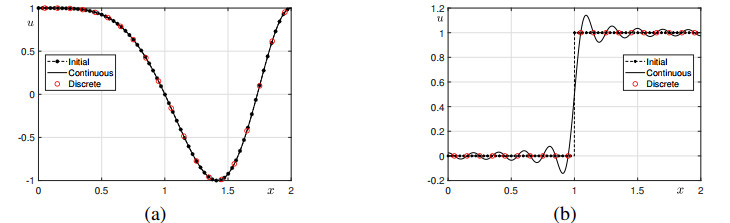
In this study, we investigate a maximum principle of the Fourier spectral method (FSM) for diffusion equations. It is well known that the FSM is fast, efficient and accurate. The maximum principle holds for diffusion equations: A solution satisfying the diffusion equation has the maximum value under the initial condition or on the boundary points. The same result can hold for the discrete numerical solution by using the FSM when the initial condition is smooth. However, if the initial condition is not smooth, then we may have an oscillatory profile of a continuous representation of the initial condition in the FSM, which can cause a violation of the discrete maximum principle. We demonstrate counterexamples where the numerical solution of the diffusion equation does not satisfy the discrete maximum principle, by presenting computational experiments. Through numerical experiments, we propose the maximum principle for the solution of the diffusion equation by using the FSM.
Citation: Junseok Kim, Soobin Kwak, Hyun Geun Lee, Youngjin Hwang, Seokjun Ham. A maximum principle of the Fourier spectral method for diffusion equations[J]. Electronic Research Archive, 2023, 31(9): 5396-5405. doi: 10.3934/era.2023273
In this study, we investigate a maximum principle of the Fourier spectral method (FSM) for diffusion equations. It is well known that the FSM is fast, efficient and accurate. The maximum principle holds for diffusion equations: A solution satisfying the diffusion equation has the maximum value under the initial condition or on the boundary points. The same result can hold for the discrete numerical solution by using the FSM when the initial condition is smooth. However, if the initial condition is not smooth, then we may have an oscillatory profile of a continuous representation of the initial condition in the FSM, which can cause a violation of the discrete maximum principle. We demonstrate counterexamples where the numerical solution of the diffusion equation does not satisfy the discrete maximum principle, by presenting computational experiments. Through numerical experiments, we propose the maximum principle for the solution of the diffusion equation by using the FSM.

| [1] |
A. Bueno-Orovio, D. Kay, K. Burrage, Fourier spectral methods for fractional-in-space reaction-diffusion equations, Bit, 54 (2014), 937–954. https://doi.org/10.1007/s10543-014-0484-2 doi: 10.1007/s10543-014-0484-2

|
| [2] | C. Canuto, Spectral methods and a maximum principle, Math. Comput., 51 (1988), 615–629. |
| [3] |
D. Li, Effective maximum principles for spectral methods, Ann. Appl. Math. 37 (2021), 131–290. https://doi.org/10.4208/aam.OA-2021-0003 doi: 10.4208/aam.OA-2021-0003
|
| [4] |
S. Lee, Non-iterative compact operator splitting scheme for Allen–Cahn equation, Comp. Appl. Math., 40 (2021), 254. https://doi.org/10.1007/s40314-021-01648-7 doi: 10.1007/s40314-021-01648-7
|
| [5] |
S. Ayub, A. Hira, S. Abdullah, Comparison of operator splitting schemes for the numerical solution of the Allen–Cahn equation, AIP Adv., 9 (2019), 125202. https://doi.org/10.1063/1.5126651 doi: 10.1063/1.5126651
|
| [6] |
S. Ham, Y. Hwang, S. Kwak, J. Kim, Unconditionally stable second-order accurate scheme for a parabolic sine-Gordon equation, AIP Adv., 12 (2022), 025203. https://doi.org/10.1063/5.0081229 doi: 10.1063/5.0081229
|
| [7] |
J. Sun, H. Zhang, X. Qian, S. Song, Up to eighth-order maximum-principle-preserving methods for the Allen–Cahn equation, Numer. Algorithms, 2022 (2022), 1–22. https://doi.org/10.1007/s11075-022-01329-4 doi: 10.1007/s11075-022-01329-4
|
| [8] |
H. G. Lee, High-order and mass conservative methods for the conservative Allen–Cahn equation, Comput. Math. Appl., 72 (2016), 620–631. https://doi.org/10.1016/j.camwa.2016.05.011 doi: 10.1016/j.camwa.2016.05.011
|
| [9] |
S. Zhai, Z. Weng, X. Feng, Investigations on several numerical methods for the non-local Allen–Cahn equation, Int. J. Heat Mass Transf., 87 (2015), 111–118. https://doi.org/10.1016/j.ijheatmasstransfer.2015.03.071 doi: 10.1016/j.ijheatmasstransfer.2015.03.071
|
| [10] |
Z. Weng, L. Tang, Analysis of the operator splitting scheme for the Allen–Cahn equation, Numer Heat Tranf. B-Fundam., 70 (2016), 472–483. https://doi.org/10.1080/10407790.2016.1215714 doi: 10.1080/10407790.2016.1215714
|
| [11] |
S. S. Alzahrani, A. Q. Khaliq, Fourier spectral exponential time differencing methods for multi-dimensional space-fractional reaction-diffusion equations, J. Comput. Appl. Math., 361 (2019), 157–175. https://doi.org/10.1016/j.cam.2019.04.001 doi: 10.1016/j.cam.2019.04.001
|
| [12] |
A. Chertock, C. R. Doering, E. Kashdan, A. Kurganov, A fast explicit operator splitting method for passive scalar advection, J. Sci. Comput., 45 (2010), 200–214. https://doi.org/10.1007/s10915-010-9381-2 doi: 10.1007/s10915-010-9381-2
|
| [13] |
M. Abbaszadeh, H. Amjadian, Second-order finite difference/spectral element formulation for solving the fractional advection-diffusion equation, Commun. Appl. Math. Comput., 2 (2020), 653–669. https://doi.org/10.1007/s42967-020-00060-y doi: 10.1007/s42967-020-00060-y
|
| [14] |
D. P. Verrall, W. W. Read, A quasi-analytical approach to the advection-diffusion-reaction problem, using operator splitting, Appl. Math. Model., 40 (2016), 1588–1598. https://doi.org/10.1016/j.apm.2015.07.023 doi: 10.1016/j.apm.2015.07.023
|
| [15] |
H. G. Lee, J. Y. Lee, A semi-analytical Fourier spectral method for the Allen–Cahn equation, Comput. Math. Appl., 68 (2014), 174–184. https://doi.org/10.1016/j.camwa.2014.05.015 doi: 10.1016/j.camwa.2014.05.015
|
| [16] |
H. Bhatt, J. Joshi, I. Argyros, Fourier spectral high-order time-stepping method for numerical simulation of the multi-dimensional Allen–Cahn equations, Symmetry, 13 (2021), 2021245. https://doi.org/10.3390/sym13020245 doi: 10.3390/sym13020245
|


Figures(5)
Junseok Kim, Soobin Kwak, Hyun Geun Lee, Youngjin Hwang, Seokjun Ham. A maximum principle of the Fourier spectral method for diffusion equations[J]. Electronic Research Archive, 2023, 31(9): 5396-5405. doi: 10.3934/era.2023273


 DownLoad: