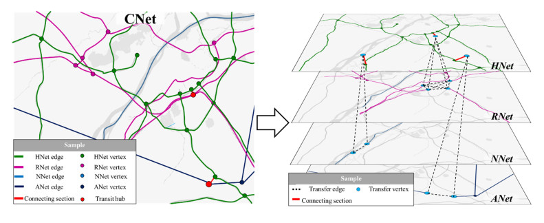
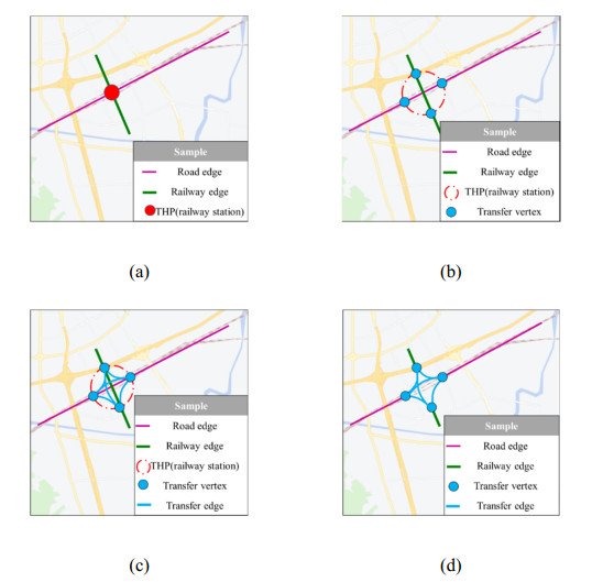
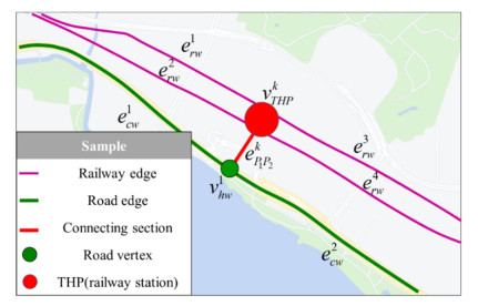
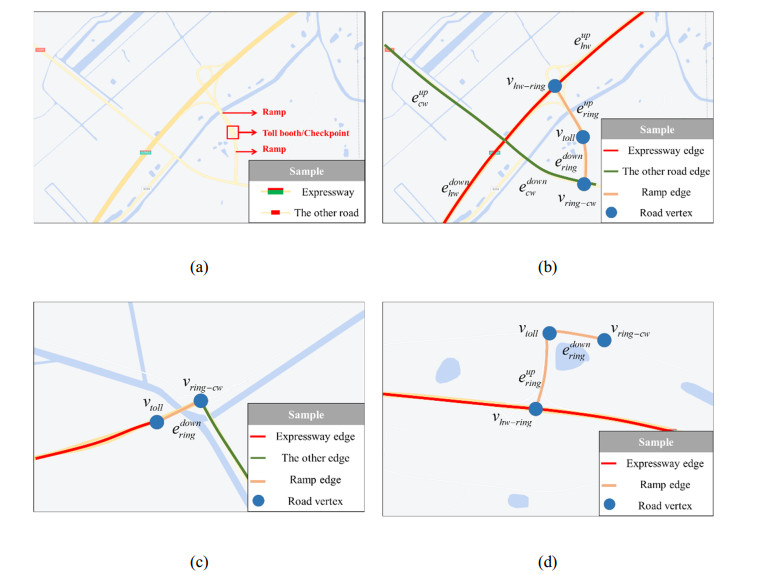
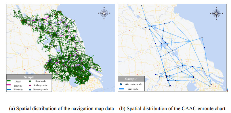
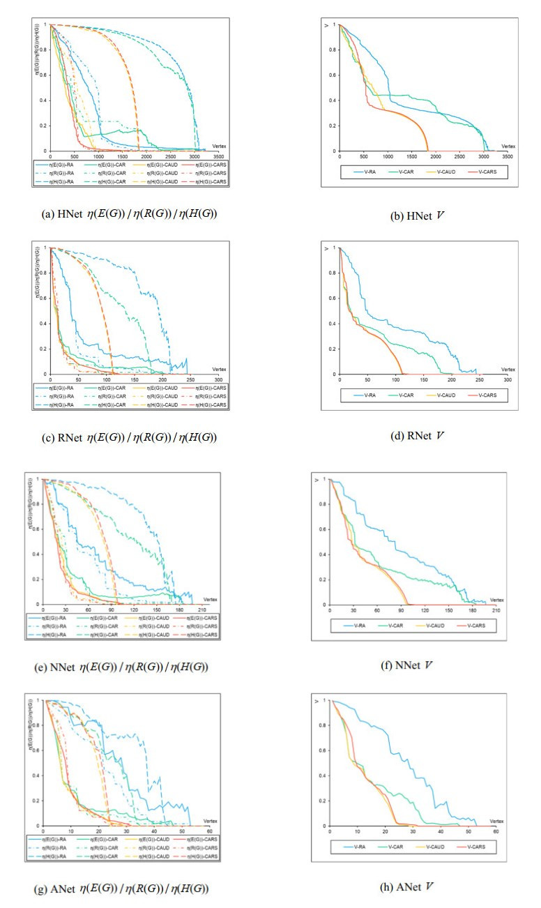
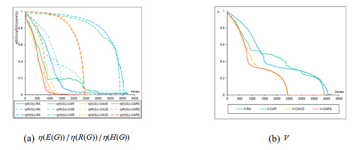
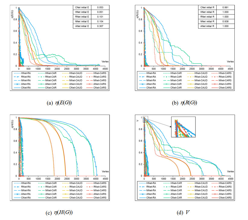
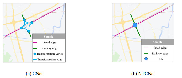
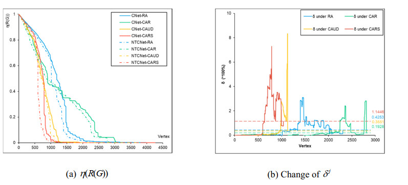
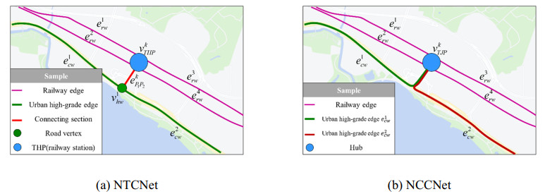
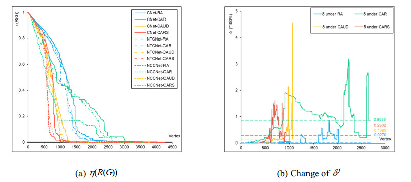
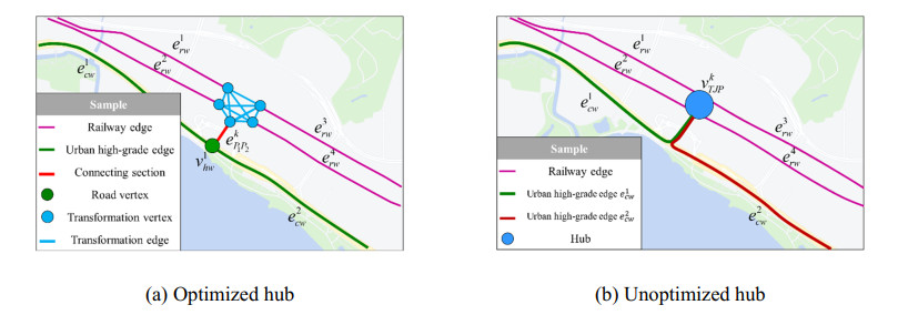
China has built a nationwide transportation network, but there needs to be a smooth connection and transfer between different modes. Five networks are constructed to explore the characteristics of a multimodal comprehensive transportation network (CNet) in Jiangsu Province based on the optimized modeling method and multisource data. Statistical and robustness characteristics are analyzed for CNet and other single-mode networks including the highway, railway, navigation channel and airway networks (HNet, RNet, NNet and ANet, respectively). The research results show following: (ⅰ) In Jiangsu, CNet, HNet, RNet and NNet are not scale-free networks and do not have small-world properties. However, ANet is the opposite. (ⅱ) The five networks in Jiangsu are robust to the random attack and their robustness changes during the attack. However, their robustness is different under different calculated attacks. For all attack strategies, CNet is the most robust. (ⅲ) In Jiangsu, the three optimized methods enhance the robustness significantly. The network failure is delayed by 12.34, 2.79 and 2.44%, respectively. The average connectivity degree is improved by 265.69, 52.95 and 32.54%, respectively. The more hubs there are with powerful transfer capacity, the stronger the network robustness. The results reveal the key points of the construction of a multimodal comprehensive transportation system and can guide the design and optimization of it.
Citation: Yongtao Zheng, Jialiang Xiao, Xuedong Hua, Wei Wang, Han Chen. A comparative analysis of the robustness of multimodal comprehensive transportation network considering mode transfer: A case study[J]. Electronic Research Archive, 2023, 31(9): 5362-5395. doi: 10.3934/era.2023272
China has built a nationwide transportation network, but there needs to be a smooth connection and transfer between different modes. Five networks are constructed to explore the characteristics of a multimodal comprehensive transportation network (CNet) in Jiangsu Province based on the optimized modeling method and multisource data. Statistical and robustness characteristics are analyzed for CNet and other single-mode networks including the highway, railway, navigation channel and airway networks (HNet, RNet, NNet and ANet, respectively). The research results show following: (ⅰ) In Jiangsu, CNet, HNet, RNet and NNet are not scale-free networks and do not have small-world properties. However, ANet is the opposite. (ⅱ) The five networks in Jiangsu are robust to the random attack and their robustness changes during the attack. However, their robustness is different under different calculated attacks. For all attack strategies, CNet is the most robust. (ⅲ) In Jiangsu, the three optimized methods enhance the robustness significantly. The network failure is delayed by 12.34, 2.79 and 2.44%, respectively. The average connectivity degree is improved by 265.69, 52.95 and 32.54%, respectively. The more hubs there are with powerful transfer capacity, the stronger the network robustness. The results reveal the key points of the construction of a multimodal comprehensive transportation system and can guide the design and optimization of it.

| [1] |
W. Wang, X. D. Hua, Y. T. Zheng, Multi-network integrated traffic analysis model and algorithm of comprehensive transportation system, J. Traffic Transp. Eng., 21 (2021), 159–172. https://doi.org/10.19818/j.cnki.1671-1637.2021.02.014 doi: 10.19818/j.cnki.1671-1637.2021.02.014

|
| [2] |
R. Albert, H. Jeong, A. L. Barabási, Internet-Diameter of the world wide web, Nature, 401 (1999), 130–131. https://doi.org/10.1136/tc.12.3.256 doi: 10.1136/tc.12.3.256
|
| [3] | A. L. Brabasi, Network Science, Cambridge University Press, Cambridge, United Kingdom, 2016. |
| [4] |
C. von Ferber, T. Holovatch, Y. Holovatch, V. Palchykov, Network harness: Metropolis public transport, Phys. A, 380 (2007), 585–591. https://doi.org/10.1016/J.PHYSA.2007.02.101 doi: 10.1016/J.PHYSA.2007.02.101
|
| [5] |
C. von Ferber, T. Holovatch, Y. Holovatch, V. Palchykov, Public transport networks: empirical analysis and modeling, Eur. Phys. J. B, 68 (2009), 261–275. https://doi.org/10.1140/EPJB/E2009-00090-X doi: 10.1140/EPJB/E2009-00090-X
|
| [6] |
F. Du, H. W. Huang, D. M. Zhang, F. Zhang, Analysis of characteristics of complex network and robustness in Shanghai metro network, Eng. J. Wuhan Univ., 49 (2016), 701–707. https://doi.org/10.14188/j.1671-8844.2016-05-010 doi: 10.14188/j.1671-8844.2016-05-010
|
| [7] |
J. Y. Lin, Y. F. Ban, Complex network topology of transportation systems, Transport Rev., 33 (2013), 658–685. https://doi.org/10.1080/01441647.2013.848955 doi: 10.1080/01441647.2013.848955
|
| [8] |
M. Kurant, P. Thiran, Extraction and analysis of traffic and topologies of transportation networks, Phys. Rev. E, 74 (2006), 036114. https://doi.org/10.1103/PhysRevE.74.036114 doi: 10.1103/PhysRevE.74.036114
|
| [9] |
S. Porta, P. Crucitti, V. Latora, The network analysis of urban: A primal approach, Environ. Plann. B: Urban Anal. City Sci., 33 (2006), 705–725. https://doi.org/10.1068/b32045 doi: 10.1068/b32045
|
| [10] | S. H. Dau, O. Milenkovic, Inference of latent network features via co-intersection representations of graphs, in 2016 IEEE International Symposium on Information Theory, (2016), 1351–1355. |
| [11] | R. Wang, X. Cai, Hierarchical structure, disassortativity and information measures of the US flight network, Chin. Phys. Lett., 22 (2005), 2715–2718. |
| [12] |
W. Li, X. Cai, Statistical analysis of airport network of China, Phys. Rev. E, 69 (2004), 046106. https://doi.org/10.1103/PhysRevE.69.046106 doi: 10.1103/PhysRevE.69.046106
|
| [13] |
P. R. V. Boas, F. A. Rodriguesa, L. D. Costa, Modeling worldwide highway networks, Phys. Lett. A, 374 (2009), 22–27. https://doi.org/10.1016/j.physleta.2009.10.028 doi: 10.1016/j.physleta.2009.10.028
|
| [14] |
C. E. Mandl, Evaluation and optimization of urban public transportation networks, Eur. J. Oper. Res., 5 (1980), 396–404. https://doi.org/10.1016/0377-2217(80)90126-5 doi: 10.1016/0377-2217(80)90126-5
|
| [15] |
V. Latora, M. Marchiori, Is Boston subway a small-world network?, Phys. A, 314 (2002), 109–113. https://doi.org/10.1016/S0378-4371(02)01089-0 doi: 10.1016/S0378-4371(02)01089-0
|
| [16] |
A. Chen, H. Yang, H. K. Lo, W. H. Tang, A capacity related reliability for transportation networks, J. Adv. Transp., 33 (1999), 183–200. https://doi.org/10.1002/atr.5670330207 doi: 10.1002/atr.5670330207
|
| [17] |
T. Y. Chen, H. L. Chang, G. H. Tzeng, Using a weight assessing model to identify route choice criteria and information effects, Transp. Res. Part A Policy Pract., 35 (2001), 197–224. https://doi.org/10.1016/S0965-8564(99)00055-5 doi: 10.1016/S0965-8564(99)00055-5
|
| [18] |
C. M. Zhang, W. Q. Wang, W. T. Li, W. L. Xiang, Analysis on regional economic characters of Lan-Xin High Speed Railway based on panel data, J. Rail Way Sci. Eng., 14 (2017), 12–18. https://doi.org/10.19713/j.cnki.43-1423/u.2017.01.003 doi: 10.19713/j.cnki.43-1423/u.2017.01.003
|
| [19] |
O. Froidh, Perspectives for a future high-speed train in the Swedish domestic travel market, J. Transp. Geogr., 16 (2008), 268–277. https://doi.org/10.1016/j.jtrangeo.2007.09.005 doi: 10.1016/j.jtrangeo.2007.09.005
|
| [20] |
M. T. Trobajo, M. V. Carriegos, Spanish airport network structure: Topological characterization, Comput. Math. Methods, 2022 (2022), 4952613. https://doi.org/10.1155/2022/4952613 doi: 10.1155/2022/4952613
|
| [21] |
Y. M. Zhou, J. W. Wang, G. Q. Huang, Efficiency and robustness of weighted air transport networks, Transp. Res. Part E Logist. Transp. Rev., 122 (2019), 14–26. https://doi.org/10.1016/j.tre.2018.11.008 doi: 10.1016/j.tre.2018.11.008
|
| [22] |
J. H. Zhang, F. N. Hu, S. L. Wang, Y. Dai, Y. X. Wang, Structural vulnerability and intervention of high speed railway networks, Phys. A, 462 (2016), 743–751. https://doi.org/10.1016/j.physa.2016.06.132 doi: 10.1016/j.physa.2016.06.132
|
| [23] |
P. Sen, S. Dasgupta, A. Chatterjee, P. A. Sreeram, G. Mukherjee, S. S. Manna, Small-world properties of the Indian railway network, Phys. Rev. E, 67 (2003), 036106. https://doi.org/10.1103/PhysRevE.67.036106 doi: 10.1103/PhysRevE.67.036106
|
| [24] |
G. Bagler, Analysis of the airport network of India as a complex weighted network, Phys. A, 387 (2008), 2972–2980. https://doi.org/10.1016/j.physa.2008.01.077 doi: 10.1016/j.physa.2008.01.077
|
| [25] |
J. Sienkiewicz, J. A. Hołyst, Statistical analysis of 22 public transport networks in Poland, Phys. Rev. E, 72 (2005), 046127. https://doi.org/10.1103/PhysRevE.72.046127 doi: 10.1103/PhysRevE.72.046127
|
| [26] | P. Marcotte, Supernetworks: Decision-making for the information age, J. Reg. Sci., 43 (2003), 615–617. |
| [27] |
S. C. Dafermos, The traffic assignment problem for multiclass-user transportation networks, Transp. Sci., 6 (1972), 73–87. https://doi.org/10.1287/trsc.6.1.73 doi: 10.1287/trsc.6.1.73
|
| [28] |
Z. X. Wu, W. H. K. Lam, Network equilibrium model for congested multi-mode transport network with elastic demand, J. Adv. Transp., 37 (2003), 295–318. https://doi.org/10.1002/atr.5670370304 doi: 10.1002/atr.5670370304
|
| [29] | P. Xu, Intercity multi-modal traffic assignment model and algorithm for urban agglomeration considering the whole travel process, in IOP Conference Series: Earth and Environmental Science, 189 (2018), 062016. https://doi.org/10.1088/1755-1315/189/6/062016 |
| [30] | H. Y. Ding, Research on Urban Multi-Modal Public Transit Network Fast Construction Method and Assignment Model, Ph.D thesis, Southeast University, 2018. |
| [31] |
A. Lozano, G. Storchi, Shortest viable path algorithm in multimodal networks, Transp. Res. Part A Policy Pract., 35 (2001), 225–241. https://doi.org/10.1016/S0965-8564(99)00056-7 doi: 10.1016/S0965-8564(99)00056-7
|
| [32] |
H. P. Shi, J. Lu, Z. Z. Yang, A super-network model based analysis of effect of comprehensive transportation polices, Logist. Technol., 31 (2012), 12–15. https://doi.org/10.3969/j.issn.1005-152X.2012.07.005 doi: 10.3969/j.issn.1005-152X.2012.07.005
|
| [33] |
G. H. Deng, M. Zhong, A. Raza, J. D. Hunt, Y. Zhou, A methodological study of multimodal freight transportation models for large regions based on an integrated modeling framework, J. Transp. Syst. Eng. Inf. Technol., 22 (2022), 30–42. https://doi.org/10.16097/j.cnki.1009-6744.2022.04.004 doi: 10.16097/j.cnki.1009-6744.2022.04.004
|
| [34] |
J. Xu, Y. N. Yin, X. Wen, G. Z. Lin, Research on the supernetwork equalization model of multilayer attributive regional logistics integration, Discrete Dyn. Nat. Soc., 2019 (2019), 8583060. https://doi.org/10.1155/2019/8583060 doi: 10.1155/2019/8583060
|
| [35] |
Y. Luo, D. L. Qian, Construction of subway and bus transport networks and analysis of the network topology characteristics, J. Transp. Syst. Eng. Inf. Technol., 15 (2015), 39–44. https://doi.org/10.16097/j.cnki.1009-6744.2015.05.006. doi: 10.16097/j.cnki.1009-6744.2015.05.006
|
| [36] |
F. Xu, J. F. Zhu, W. D. Yang, Construction of high-speed railway and airline compound network and the analysis of its network topology characteristics, Complex Syst. Complexity Sci., 10 (2013), 1–11. https://doi.org/10.13306/j.1672-3813.2013.03.001 doi: 10.13306/j.1672-3813.2013.03.001
|
| [37] |
X. Feng, S. W. He, G. Y. Li, J. S. Chi, Transfer network of high-speed rail and aviation: Structure and critical components, Phys. A, 581 (2021), 126197. https://doi.org/10.1016/j.physa.2021.126197 doi: 10.1016/j.physa.2021.126197
|
| [38] |
M. Ouyang, Z. Z. Pan, L. Hong, Y. He, Vulnerability analysis of complementary transportation systems with applications to railway and airline systems in China, Reliab. Eng. Syst. Saf., 142 (2015), 248–257. https://doi.org/10.1016/j.ress.2015.05.013 doi: 10.1016/j.ress.2015.05.013
|
| [39] |
Y. Luo, D. L. Qian, Construction of subway and bus transport networks and analysis of the network topology characteristics, J. Transp. Syst. Eng. Inf. Technol., 15(2015), 39–44. https://doi.org/10.16097/j.cnki.1009-6744.2015.05.006 doi: 10.16097/j.cnki.1009-6744.2015.05.006
|
| [40] |
X. H. Li, J. Y. Guo, C. Gao, Z. Su, D. Bao, Z. L. Zhang, Network-based transportation system analysis: A case study in a mountain city, Chaos, Solitons Fractals, 107 (2018), 256–265. https://doi.org/10.1016/j.chaos.2 doi: 10.1016/j.chaos.2
|
| [41] |
G. Liu, Y. S. Li, Robustness analysis of railway transer system based on complex network theory, Appl. Res. Comput., 31 (2014), 2941–2942, 2973. https://doi.org/10.3969/j.issn.1001-3695.2014.10.013 doi: 10.3969/j.issn.1001-3695.2014.10.013
|
| [42] |
S. Wandelt, X. Shi, X. Q. Sun, Estimation and improvement of transportation network robustness by exploiting communities, Reliab. Eng. Syst. Saf., 206 (2021), 107307. https://doi.org/10.1016/j.ress.2020.107307 doi: 10.1016/j.ress.2020.107307
|
| [43] |
M. Barthélemy, Betweenness centrality in large complex networks, Eur. Phys. J. B, 38 (2004), 163–168. https://doi.org/10.1140/epjb/e2004-00111-4 doi: 10.1140/epjb/e2004-00111-4
|
| [44] |
U. Demšar, O. Špatenková, K. Virrantaus, Identifying critical locations in a spatial network with graph theory, Trans. GIS, 12 (2008), 61–82. https://doi.org/10.1111/j.1467-9671.2008.01086.x doi: 10.1111/j.1467-9671.2008.01086.x
|
| [45] |
Y. S. Chen, X. Y. Wang, X. W. Song, J. L. Jia, Y. Y. Chen, W. L. Shang, Resilience assessment of multimodal urban transport networks, J. Circuits Syst. Comput., 31 (2022), 18. https://doi.org/10.1142/S0218126622503108 doi: 10.1142/S0218126622503108
|
| [46] |
Y. Y. Duan, F. Lu, Robustness of city road networks at different granularities, Phys. A, 411 (2014), 21–34. https://doi.org/10.1016/j.physa.2014.05.073 doi: 10.1016/j.physa.2014.05.073
|
| [47] |
F. Morone, H. A. Makse, Influence maximization in complex networks through optimal percolation, Nature, 524 (2015), 65–68. https://doi.org/10.1038/nature14604 doi: 10.1038/nature14604
|
| [48] |
L. Zdeborová, P. Zhang, H. J. Zhou, Fast and simple decycling and dismantling of networks, Sci. Rep., 6 (2016), 37953. https://doi.org/10.1038/srep37954 doi: 10.1038/srep37954
|
| [49] |
O. Cats, G. J. Koppenol, M. Warnier, Robustness assessment of link capacity reduction for complex networks: Application for public transport systems, Reliab. Eng. Syst. Saf., 167 (2017), 544–553. https://doi.org/10.1016/j.ress.2017.07.009 doi: 10.1016/j.ress.2017.07.009
|
| [50] |
W. L. Shang, Z. Y. Gao, N. Daina, H. R. Zhang, Y. Long, Z. L. Guo, et al., Benchmark analysis for robustness of multi-scale urban road networks under global disruptions, IEEE Trans. Intell. Transp. Syst., 2022 (2022). https://doi.org/10.1109/TITS.2022.3149969 doi: 10.1109/TITS.2022.3149969
|
| [51] |
M. Ouyang, C. Liu, M. Xu, Value of resilience-based solutions on critical infrastructure protection: Comparing with robustness-based solutions, Reliab. Eng. Syst. Saf., 190 (2019), 106506. https://doi.org/10.1016/j.ress.2019.106506 doi: 10.1016/j.ress.2019.106506
|
| [52] |
A. Kermanshah, S. Derrible, A geographical and multi-criteria vulnerability assessment of transportation networks against extreme earthquakes, Reliab. Eng. Syst. Saf., 153 (2016), 39–49. https://doi.org/10.1016/j.ress.2016.04.007 doi: 10.1016/j.ress.2016.04.007
|
| [53] |
W. L. Shang, Y. Y. Chen, C. C. Song, W. Y. Ochieng, Robustness analysis of urban road networks from topological and operational perspectives, Math. Probl. Eng., 2020 (2020), 5875803. https://doi.org/10.1155/2020/5875803 doi: 10.1155/2020/5875803
|
| [54] |
Z. Z. Liu, H. Chen, E. Z. Liu, W. Y. Hu, Exploring the resilience assessment framework of urban road network for sustainable cities, Phys. A, 586 (2022), 126465. https://doi.org/10.1016/j.physa.2021.126465 doi: 10.1016/j.physa.2021.126465
|
| [55] |
Y. F. Zhang, S. T. Ng, Robustness of urban railway networks against the cascading failures induced by the fluctuation of passenger flow, Reliab. Eng. Syst. Saf., 219 (2022), 108227. https://doi.org/10.1016/j.ress.2021.108227 doi: 10.1016/j.ress.2021.108227
|
| [56] |
Y. Chen, J. E. Wang, F. J. Jin, Robustness of China's air transport network from 1975 to 2017, Phys. A, 539 (2020), 122876. https://doi.org/10.1016/j.physa.2019.122876 doi: 10.1016/j.physa.2019.122876
|
| [57] |
T. Li, L. L. Rong, K. S. Yan, Vulnerability analysis and critical area identification of public transport system: A case of high-speed rail and air transport coupling system in China, Transp. Res. Part A Policy Pract., 127 (2019), 55–70. https://doi.org/10.1016/j.tra.2019.07.008 doi: 10.1016/j.tra.2019.07.008
|
| [58] | Available from: https://navinfo.com/en/aboutus. |
| [59] | Air Traffic Management Office, Specifications for the Compilation and Drawing of Civil Aviation Instrument Route Charts and Area Charts, Available from: http://www.caac.gov.cn/XXGK/XXGK/GFXWJ/202111/t20211130_210338.html. |
| [60] |
H. Li, L. X. Gan, Y. Z. Zheng, Y. Q. Wen, Complexity of waterway networks in port waters, J. Navig. China, 38 (2015), 94–98, 130. https://doi.org/10.3969/j.issn.1000-4653.2015.03.021 doi: 10.3969/j.issn.1000-4653.2015.03.021
|
| [61] |
N. Y. Lou, C. H. Huang, Y. L. Chen, Y. Luan, J. H. Yuan, Network characteristics and robustness analysis of high level waterway network in the Yangtze River Delta, J. Dalian Marit. Univ., 47 (2021), 28–36. https://doi.org/10.16411/j.cnki.issn1006-7736.2021.01.004. doi: 10.16411/j.cnki.issn1006-7736.2021.01.004
|
| [62] |
B. B. Fu, Z. Y. Gao, F. S. Liu, X. J. Kong, Express passenger transport system as a scale-free network, Mod. Phys. Lett. B, 20 (2006), 1755–1761. https://doi.org/10.1142/S0217984906011803 doi: 10.1142/S0217984906011803
|
| [63] |
W. Zhao, H. S. He, Z. C. Lin, K. Q. Yang, The study of properties of Chinese railway passenger transport network, Acta Phys. Sin., 55 (2006), 3906–3911. https://doi.org/10.7498/aps.55.3906 doi: 10.7498/aps.55.3906
|
| [64] |
L. N. Wu, Y. F. Lyu, Y. S. Ci, Connectivity reliability for provincial freeway network: A case study in Heilongjiang, China, J. Transp. Syst. Eng. Inf. Technol., 18 (2018), 134–140. https://doi.org/10.16097/j.cnki.1009-6744.2018.Sup.1.020 doi: 10.16097/j.cnki.1009-6744.2018.Sup.1.020
|
Figures(20) / Tables(8)
Yongtao Zheng, Jialiang Xiao, Xuedong Hua, Wei Wang, Han Chen. A comparative analysis of the robustness of multimodal comprehensive transportation network considering mode transfer: A case study[J]. Electronic Research Archive, 2023, 31(9): 5362-5395. doi: 10.3934/era.2023272


 DownLoad: