Using deep learning in pathology image analysis: A novel active learning strategy based on latent representation

Yixin Sun; Lei Wu; Peng Chen; Feng Zhang; Lifeng Xu; Yixin Sun; Lei Wu; Peng Chen; Feng Zhang; Lifeng Xu

doi:10.3934/era.2023271

Electronic Research Archive

2023, Volume 31, Issue 9: 5340-5361. doi: 10.3934/era.2023271

Previous Article Next Article

Research article Special Issues

Using deep learning in pathology image analysis: A novel active learning strategy based on latent representation

1.
School of Mathematical Sciences, University of Electronic Science and Technology of China, Chengdu 611731, China
2.
Yangtze Delta Region Institute (Quzhou), University of Electronic Science and Technology of China, Quzhou 314099, China
3.
School of Computer and Software Engineering, Xihua University, Chengdu 611731, China
4.
The Quzhou Affiliated Hospital of Wenzhou Medical University, Quzhou People's Hospital, Quzhou 324000, China

Received: 23 May 2023 Revised: 10 July 2023 Accepted: 11 July 2023 Published: 27 July 2023

Most countries worldwide continue to encounter a pathologist shortage, significantly impeding the timely diagnosis and effective treatment of cancer patients. Deep learning techniques have performed remarkably well in pathology image analysis; however, they require expert pathologists to annotate substantial pathology image data. This study aims to minimize the need for data annotation to analyze pathology images. Active learning (AL) is an iterative approach to search for a few high-quality samples to train a model. We propose our active learning framework, which first learns latent representations of all pathology images by an auto-encoder to train a binary classification model, and then selects samples through a novel ALHS (Active Learning Hybrid Sampling) strategy. This strategy can effectively alleviate the sample redundancy problem and allows for more informative and diverse examples to be selected. We validate the effectiveness of our method by undertaking classification tasks on two cancer pathology image datasets. We achieve the target performance of 90% accuracy using 25% labeled samples in Kather's dataset and reach 88% accuracy using 65% labeled data in BreakHis dataset, which means our method can save 75% and 35% of the annotation budget in the two datasets, respectively.
- active learning,
- pathology images classification,
- latent representation,
- samples selection,
- ALHS strategy
Citation: Yixin Sun, Lei Wu, Peng Chen, Feng Zhang, Lifeng Xu. Using deep learning in pathology image analysis: A novel active learning strategy based on latent representation[J]. Electronic Research Archive, 2023, 31(9): 5340-5361. doi: 10.3934/era.2023271

Related Papers:

Abstract

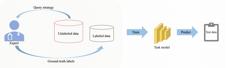
Most countries worldwide continue to encounter a pathologist shortage, significantly impeding the timely diagnosis and effective treatment of cancer patients. Deep learning techniques have performed remarkably well in pathology image analysis; however, they require expert pathologists to annotate substantial pathology image data. This study aims to minimize the need for data annotation to analyze pathology images. Active learning (AL) is an iterative approach to search for a few high-quality samples to train a model. We propose our active learning framework, which first learns latent representations of all pathology images by an auto-encoder to train a binary classification model, and then selects samples through a novel ALHS (Active Learning Hybrid Sampling) strategy. This strategy can effectively alleviate the sample redundancy problem and allows for more informative and diverse examples to be selected. We validate the effectiveness of our method by undertaking classification tasks on two cancer pathology image datasets. We achieve the target performance of 90% accuracy using 25% labeled samples in Kather's dataset and reach 88% accuracy using 65% labeled data in BreakHis dataset, which means our method can save 75% and 35% of the annotation budget in the two datasets, respectively.

References

[1]	H. Sung, J. Ferlay, R. L. Siegel, M. Laversanne, I. Soerjomataram, A. Jemal, et al., Global cancer statistics 2020: Globocan estimates of incidence and mortality worldwide for 36 cancers in 185 countries, CA: Cancer J. Clin., 71 (2021), 209–249. https://doi.org/10.3322/caac.21660 doi: 10.3322/caac.21660
[2]	J. Ferlay, M. Colombet, I. Soerjomataram, D. M. Parkin, M. Piñeros, A. Znaor, et al., Cancer statistics for the year 2020: An overview, Int. J. Cancer, 149 (2021), 778–789. https://doi.org/10.1002/ijc.33588 doi: 10.1002/ijc.33588
[3]	B. Acs, M. Rantalainen, J. Hartman, Artificial intelligence as the next step towards precision pathology, J. Int. Med., 288 (2020), 62–81. https://doi.org/10.1111/joim.13030 doi: 10.1111/joim.13030
[4]	E. J. Topol, High-performance medicine: The convergence of human and artificial intelligence, Nat. Med., 25 (2019), 44–56. https://doi.org/10.1038/s41591-018-0300-7 doi: 10.1038/s41591-018-0300-7
[5]	D. M. Metter, T. J. Colgan, S. T. Leung, C. F. Timmons, J. Y. Park, Trends in the us and canadian pathologist workforces from 2007 to 2017, JAMA Netw. Open, 2 (2019), e194337. https://doi.org/10.1001/jamanetworkopen.2019.4337 doi: 10.1001/jamanetworkopen.2019.4337
[6]	Y. Song, R. Xin, P. Chen, R. Zhang, J. Chen, Z. Zhao, Identifying performance anomalies in fluctuating cloud environments: A robust correlative-gnn-based explainable approach, Future Gener. Comput. Syst., 145 (2023), 77–86.
[7]	T. Xie, X. Cheng, X. Wang, M. Liu, J. Deng, T. Zhou, et al., Cut-thumbnail: A novel data augmentation for convolutional neural network, in Proceedings of the 29th ACM International Conference on Multimedia, (2021), 1627–1635.
[8]	H. Liu, P. Chen, X. Ouyang, G. Hui, Y. Bing, P. Grosso, et al., Robustness challenges in reinforcement learning based time-critical cloud resource scheduling: A meta-learning based solution, Future Gener. Comput. Syst., 146 (2023), 18–33. https://doi.org/10.1016/j.future.2023.03.029 doi: 10.1016/j.future.2023.03.029
[9]	H. Lu, X. Cheng, W. Xia, P. Deng, M. Liu, T. Xie, et al., Cyclicshift: A data augmentation method for enriching data patterns, in Proceedings of the 30th ACM International Conference on Multimedia, (2022), 4921–4929.
[10]	P. Chen, H. Liu, R. Xin, T. Carval, J. Zhao, Y. Xia, et al., Effectively detecting operational anomalies in large-scale IoT data infrastructures by using a GAN-based predictive model, Comput. J., 65 (2022), 2909–2925.
[11]	C. Janiesch, P. Zschech, K. Heinrich, Machine learning and deep learning, Electron. Mark., 31 (2021), 685–695. https://doi.org/10.1007/s12525-021-00475-2 doi: 10.1007/s12525-021-00475-2
[12]	A. L. Yuille, C. Liu, Deep nets: What have they ever done for vision, Int. J. Comput. Vision, 129 (2021), 781–802. https://doi.org/10.1007/s11263-020-01405-z doi: 10.1007/s11263-020-01405-z
[13]	Z. H. Zhou, A brief introduction to weakly supervised learning, Natl. Sci. Rev., 5 (2017), 44–53, https://doi.org/10.1093/nsr/nwx106 doi: 10.1093/nsr/nwx106
[14]	O. Sener, S. Savarese, Active learning for convolutional neural networks: A core-set approach, arXiv preprint, (2017), arXiv: 1708.00489. https://doi.org/10.48550/arXiv.1708.00489
[15]	N. Houlsby, F. Huszár, Z. Ghahramani, M. Lengyel, Bayesian active learning for classification and preference learning, arXiv preprint, (2011), arXiv: 1112.5745. https://doi.org/10.48550/arXiv.1112.5745
[16]	S. Sinha, S. Ebrahimi, T. Darrell, Variational adversarial active learning, in 2019 IEEE/CVF International Conference on Computer Vision (ICCV), Seoul, Korea, (2019), 5971–5980. https://doi.org/10.1109/ICCV.2019.00607
[17]	A. Halder, A. Kumar, Active learning using rough fuzzy classifier for cancer prediction from microarray gene expression data, J. Biomed. Inf., 92 (2019), 103136. https://doi.org/10.1016/j.jbi.2019.103136 doi: 10.1016/j.jbi.2019.103136
[18]	D. Mahapatra, B. Bozorgtabar, J. P. Thiran, M. Reyes, Efficient active learning for image classification and segmentation using a sample selection and conditional generative adversarial network, in International Conference on Medical Image Computing and Computer-Assisted Intervention, Springer International Publishing, (2018), 580–588. https://doi.org/10.3917/perri.berli.2018.01.0580
[19]	A. L. Meirelles, T. Kurc, J. Saltz, G. Teodoro, Effective active learning in digital pathology: A case study in tumor infiltrating lymphocytes, Comput. Methods Programs Biomed., 220 (2022), 106828.
[20]	A. Culotta, A. McCallum, Reducing labeling effort for structured prediction tasks, in AAAI, 5 (2005), 746–751.
[21]	T. Scheffer, C. Decomain, S. Wrobel, Active hidden markov models for information extraction, in International Symposium on Intelligent Data Analysis (IDA), Springer, Cascais, Portugal, (2001), 309–318.
[22]	C. E. Shannon, A mathematical theory of communication, ACM SIGMOBILE Mobile Comput. Commun. Rev., 5 (2001), 3–55. https://doi.org/10.1145/584091.584093 doi: 10.1145/584091.584093
[23]	J. N. Kather, C. A. Weis, F. Bianconi, S. M. Melchers, L. R. Schad, T. Gaiser, et al., Multi-class texture analysis in colorectal cancer histology, Sci. Rep., 6 (2016), 1–11. https://doi.org/10.1038/srep27988 doi: 10.1038/srep27988
[24]	F. A. Spanhol, L. S. Oliveira, C. Petitjean, L. Heutte, A dataset for breast cancer histopathological image classification, IEEE Trans. Biomed. Eng., 63 (2015), 1455–1462. https://doi.org/10.1109/TBME.2015.2496264 doi: 10.1109/TBME.2015.2496264
[25]	K. He, X. Zhang, S. Ren, J. Sun, Deep residual learning for image recognition, in 2016 IEEE Conference on Computer Vision and Pattern Recognition (CVPR), IEEE, Las Vegas, USA, (2016), 770–778.
[26]	D. Gissin, S. Shalev-Shwartz, Discriminative active learning, arXiv preprint, (2019), arXiv: 1907.06347. https://doi.org/10.48550/arXiv.1907.06347
[27]	L. Van der Maaten, G. Hinton, Visualizing data using t-sne, J. Mach. Learn. Res., 9 (2008), 2579–2605.
[28]	T. Ching, D. S. Himmelstein, B. K. Beaulieu-Jones, A. A. Kalinin, B. T. Do, G. P. Way, et al., Opportunities and obstacles for deep learning in biology and medicine, J. R. Soc. Interface, 15 (2018), 20170387.
[29]	S. Nanga, A. T. Bawah, B. A. Acquaye, M. I. Billa, F. D. Baeta, N. A. Odai, et al., Review of dimension reduction methods, J. Data Anal. Inf. Process., 9 (2021), 189–231. https://doi.org/10.4236/jdaip.2021.93013 doi: 10.4236/jdaip.2021.93013
[30]	A. L'Heureux, K. Grolinger, H. F. Elyamany, M. A. M. Capretz, Machine learning with big data: Challenges and approaches, IEEE Access, 5 (2017), 7776–7797. https://doi.org/10.1109/ACCESS.2017.2696365 doi: 10.1109/ACCESS.2017.2696365
[31]	A. Bria, C. Marrocco, F. Tortorella, Addressing class imbalance in deep learning for small lesion detection on medical images, Comput. Biol. Med., 120 (2020), 103735. https://doi.org/10.1016/j.compbiomed.2020.103735 doi: 10.1016/j.compbiomed.2020.103735
[32]	M. Outtas, Compression Oriented Enhancement of Noisy Images: Application to Ultrasound Images, USTHB-Alger, 2019.
[33]	C. Doersch, Tutorial on variational autoencoders, arXiv preprint, (2016), arXiv: 1606.05908. https://doi.org/10.48550/arXiv.1606.05908
[34]	I. Goodfellow, J. Pouget-Abadie, M. Mirza, B. Xu, D. Warde-Farley, S. Ozair, et al., Generative adversarial networks, Commun. ACM, 63 (2020), 139–144. https://doi.org/10.1145/3422622 doi: 10.1145/3422622
[35]	M. Mirza, S. Osindero, Conditional generative adversarial nets, arXiv preprint, (2014), arXiv: 1411.1784. https://doi.org/10.48550/arXiv.1411.1784
[36]	I. Gulrajani, F. Ahmed, M. Arjovsky, V. Dumoulin, A. C. Courville, Improved training of wasserstein gans, in Advances in Neural Information Processing Systems, (2017), 5769–5779.
[37]	J. Y. Zhu, T. Park, P. Isola, A. A. Efros, Unpaired image-to-image translation using cycle-consistent adversarial networks, in Proceedings of the IEEE International Conference on Computer Vision (ICCV), IEEE, Venice, Italy, (2017), 2242–2251.
[38]	A. Brock, J. Donahue, K. Simonyan, Large scale gan training for high fidelity natural image synthesis, arXiv preprint, (2018), arXiv: 1809.11096. https://doi.org/10.48550/arXiv.1809.11096
[39]	J. Zhao, M. Mathieu, Y. LeCun, Energy-based generative adversarial network, arXiv preprint, (2016), arXiv: 1609.03126. https://doi.org/10.48550/arXiv.1609.03126
[40]	S. Qiao, W. Shen, Z. Zhang, B. Wang, A. Yuille, Deep co-training for semi-supervised image recognition, in Proceedings of the European Conference on Computer Vision (ECCV), Munich, Germany, (2018), 142–159. https://doi.org/10.1787/qna-v2018-2-12-en
[41]	H. Pham, Z. Dai, Q. Xie, Q. V. Le, Meta pseudo labels, in Proceedings of the IEEE/CVF Conference on Computer Vision and Pattern Recognition (CVPR), Nashville, USA, (2021), 11557–11568.
[42]	X. Wang, D. Kihara, J. Luo, G. J. Qi, Enaet: A self-trained framework for semi-supervised and supervised learning with ensemble transformations, IEEE Trans. Image Process., 30 (2021), 1639–1647. https://doi.org/10.1109/TIP.2020.3044220 doi: 10.1109/TIP.2020.3044220
[43]	Y. Lecun, L. Bottou, Y. Bengio, P. Haffner, Gradient-based learning applied to document recognition, Proc. IEEE, 86 (1998), 2278–2324. https://doi.org/10.1109/5.726791 doi: 10.1109/5.726791
[44]	A. Krizhevsky, G. Hinton, Learning multiple layers of features from tiny images, 2009 (2009), 1–58.
[45]	J. Deng, W. Dong, R. Socher, L. J. Li, K. Li, L. Fei-Fei, Imagenet: A large-scale hierarchical image database, in Proceedings of the IEEE Conference on Computer Vision and Pattern Recognition (CVPR), IEEE Computer Society, Los Alamitos, USA, (2009), 248–255.
[46]	M. Versaci, G. Angiulli, P. Crucitti, D. De Carlo, F. Laganà, D. Pellicanò, et al., A fuzzy similarity-based approach to classify numerically simulated and experimentally detected carbon fiber-reinforced polymer plate defects, Sensors, 22, (2022), 4232. https://doi.org/10.3390/s22114232
[47]	A. T. Azar, A. E. Hassanien, Dimensionality reduction of medical big data using neural-fuzzy classifier, Soft comput., 19 (2015), 1115–1127. https://doi.org/10.1007/s00500-014-1327-4 doi: 10.1007/s00500-014-1327-4
[48]	N. Lei, Y. Guo, D. An, X. Qi, Z. Luo, S. T. Yau, et al., Mode collapse and regularity of optimal transportation maps, arXiv preprint, (2019), arXiv: 1902.02934. https://doi.org/10.48550/arXiv.1902.02934
[49]	M. Arjovsky, L. Bottou, Towards principled methods for training generative adversarial networks, in International Conference on Learning Representations(ICLR), Toulon, France, (2017), 1–17.

Reader Comments

Your name:*

Email:*
© 2023 the Author(s), licensee AIMS Press. This is an open access article distributed under the terms of the Creative Commons Attribution License (http://creativecommons.org/licenses/by/4.0)