This manuscript is devoted to presenting some convergence results of a three-step iterative scheme under the Chatterjea–Suzuki–C ((CSC), for short) condition in the setting of a Banach space. Also, an example of mappings satisfying the (CSC) condition with a unique fixed point is provided. This example proves that the proposed scheme converges to a fixed point of a weak contraction faster than some known and leading schemes. Finally, our main results will be applied to find a solution to functional and fractional differential equations (FDEs) as an application.
Citation: Junaid Ahmad, Kifayat Ullah, Hasanen A. Hammad, Reny George. A solution of a fractional differential equation via novel fixed-point approaches in Banach spaces[J]. AIMS Mathematics, 2023, 8(6): 12657-12670. doi: 10.3934/math.2023636
| [1] | Ahmed M.A. El-Sayed, Eman M.A. Hamdallah, Hameda M. A. Alama . Multiple solutions of a Sturm-Liouville boundary value problem of nonlinear differential inclusion with nonlocal integral conditions. AIMS Mathematics, 2022, 7(6): 11150-11164. doi: 10.3934/math.2022624 |
| [2] | Murugesan Manigandan, Kannan Manikandan, Hasanen A. Hammad, Manuel De la Sen . Applying fixed point techniques to solve fractional differential inclusions under new boundary conditions. AIMS Mathematics, 2024, 9(6): 15505-15542. doi: 10.3934/math.2024750 |
| [3] | Mouffak Benchohra, John R. Graef, Nassim Guerraiche, Samira Hamani . Nonlinear boundary value problems for fractional differential inclusions with Caputo-Hadamard derivatives on the half line. AIMS Mathematics, 2021, 6(6): 6278-6292. doi: 10.3934/math.2021368 |
| [4] | Bashir Ahmad, Badrah Alghamdi, Ahmed Alsaedi, Sotiris K. Ntouyas . Existence results for Riemann-Liouville fractional integro-differential inclusions with fractional nonlocal integral boundary conditions. AIMS Mathematics, 2021, 6(7): 7093-7110. doi: 10.3934/math.2021416 |
| [5] | Madeaha Alghanmi, Shahad Alqurayqiri . Existence results for a coupled system of nonlinear fractional functional differential equations with infinite delay and nonlocal integral boundary conditions. AIMS Mathematics, 2024, 9(6): 15040-15059. doi: 10.3934/math.2024729 |
| [6] | Abdissalam Sarsenbi, Abdizhahan Sarsenbi . Boundary value problems for a second-order differential equation with involution in the second derivative and their solvability. AIMS Mathematics, 2023, 8(11): 26275-26289. doi: 10.3934/math.20231340 |
| [7] | Adel Lachouri, Mohammed S. Abdo, Abdelouaheb Ardjouni, Bahaaeldin Abdalla, Thabet Abdeljawad . On a class of differential inclusions in the frame of generalized Hilfer fractional derivative. AIMS Mathematics, 2022, 7(3): 3477-3493. doi: 10.3934/math.2022193 |
| [8] | Djamila Chergui, Taki Eddine Oussaeif, Merad Ahcene . Existence and uniqueness of solutions for nonlinear fractional differential equations depending on lower-order derivative with non-separated type integral boundary conditions. AIMS Mathematics, 2019, 4(1): 112-133. doi: 10.3934/Math.2019.1.112 |
| [9] | Nayyar Mehmood, Niaz Ahmad . Existence results for fractional order boundary value problem with nonlocal non-separated type multi-point integral boundary conditions. AIMS Mathematics, 2020, 5(1): 385-398. doi: 10.3934/math.2020026 |
| [10] | Najla Alghamdi, Bashir Ahmad, Esraa Abed Alharbi, Wafa Shammakh . Investigation of multi-term delay fractional differential equations with integro-multipoint boundary conditions. AIMS Mathematics, 2024, 9(5): 12964-12981. doi: 10.3934/math.2024632 |
This manuscript is devoted to presenting some convergence results of a three-step iterative scheme under the Chatterjea–Suzuki–C ((CSC), for short) condition in the setting of a Banach space. Also, an example of mappings satisfying the (CSC) condition with a unique fixed point is provided. This example proves that the proposed scheme converges to a fixed point of a weak contraction faster than some known and leading schemes. Finally, our main results will be applied to find a solution to functional and fractional differential equations (FDEs) as an application.
The models of the differential and integral equations have been appeared in different applications (see [1,2,3,4,6,7,9,12,13,14,15,16,17,18,19,20]).
Boundary value problems involving fractional differential equations arise in physical sciences and applied mathematics. In some of these problems, subsidiary conditions are imposed locally. In some other cases, nonlocal conditions are imposed. It is sometimes better to impose nonlocal conditions since the measurements needed by a nonlocal condition may be more precise than the measurement given by a local condition. Consequently, a variety of excellent results on fractional boundary value problems (abbreviated BVPs) with resonant conditions have been achieved. For instance, Bai [4] studied a type of fractional differential equations with m-points boundary conditions. The existence of nontrivial solutions was established by using coincidence degree theory. Applying the same method, Kosmatov [17] investigated the fractional order three points BVP with resonant case.
Although the study of fractional BVPs at resonance has acquired fruitful achievements, it should be noted that such problems with Riemann-Stieltjes integrals are very scarce, so it is worthy of further explorations. Riemann-Stieltjes integral has been considered as both multipoint and integral in a single framework, which is more common, see the relevant works due to Ahmad et al. [1].
The boundary value problems with nonlocal, integral and infinite points boundary conditions have been studied by some authors (see, for example [8,10,11,12]).
Here, we discuss the boundary value problem of the nonlinear differential inclusions of arbitrary (fractional) orders
| dxdt∈F1(t,x(t),Iγf2(t,Dαx(t))),α,γ∈(0,1]t∈(0,1) | (1.1) |
with the nonlocal boundary condition
| m∑k=1akx(τk)=x0,ak>0τk∈[0,1], | (1.2) |
the integral condition
| ∫10x(s)dg(s)=x0 | (1.3) |
and the infinite point boundary condition
| ∞∑k=1akx(τk)=x0,ak>0andτk∈[0,1]. | (1.4) |
We study the existence of solutions x∈C[0,1] of the problems (1.1) and (1.2), and deduce the existence of solutions of the problem of (1.1) with the conditions (1.3) and (1.4). Then the existence of the maximal and minimal solutions will be proved. The sufficient condition for the uniqueness and continuous dependence of the solution will be studied.
This paper is organised as: In Section 2, we prove the existence of continuous solutions of the problems (1.1) and (1.2), and deduce the existence of solutions of the problem of (1.1) with the conditions (1.3) and (1.4). In Section 3, the existence of the maximal and minimal solutions is proved. In Section 4, the sufficient condition for the uniqueness and continuous dependence of the solution are studied. Next, in Section 5, we extend our results to the nonlocal problems (1.3) and (2.1). Finally, some existence results is proved for the nonlocal problems (1.4) and (2.1) in Section 6.
Consider the following assumptions:
(I) (i) The set F1(t,x,y) is nonempty, closed and convex for all (t,x,y)∈[0,1]×R×R.
(ii) F1(t,x,y) is measurable in t∈[0,1] for every x,y∈R.
(iii) F1(t,x,y) is upper semicontinuous in x and y for every t∈[0,1].
(iv) There exist a bounded measurable function a1:[0,1]⟶R and a positive constant K1, such that
| ‖F1(t,x,y)‖=sup{|f1|:f1∈F1(t,x,y)}≤|a1(t)|+K1(|x|+|y|). |
Remark 2.1. From the assumptions (i)–(iv) we can deduce that (see [3,6,7,13]) there exists f1∈F1(t,x,y), such that
(v) f1:[0,1]×R×R⟶R is measurable in t for every x,y∈R and continuous in x,y for t∈[0,1], and there exist a bounded measurable function a1:[0,1]→R and a positive constant K1>0 such that
| |f1(t,x,y)|≤|a1(t)|+K1(|x|+|y|), |
and the functional f1 satisfies the differential equation
| dxdt=f1(t,x(t),Iγf2(t,Dαx(t))),α,γ∈(0,1]andt∈(0,1]. | (2.1) |
(II) f2:[0,1]×R⟶R is measurable in t for any x∈R and continuous in x for t∈[0,1], and there exist a bounded measurable function a2:[0,1]→R and a positive constant K2>0 such that
| |f2(t,x)|≤|a2(t)|+K2|x|,∀t∈[0,1]andx∈R |
and
| supt∈[0,1]|ai(t)|≤ai,i=1,2. |
(III) 2K1γ+K1K2α<αγΓ(2−α),α,γ∈(0,1].
Remark 2.2. From (I) and (v) we can deduce that every solution of (1.1) is a solution of (2.1). Now, we shall prove the following lemma.
Lemma 2.1. If the solution of the problems (1.2)–(2.1) exists then it can be expressed by the integral equation
| y(t)=∫t0(t−s)−αΓ(1−α)f1(s,1m∑k=1ak[x0−m∑k=1ak∫τk0(τk−θ)α−1Γ(α)y(θ)dθ]+∫s0(s−θ)α−1Γ(α)y(θ)dθ,∫s0(s−θ)γ−1Γ(γ)f2(ϕ,y(θ))dθ)ds. | (2.2) |
Proof. Consider the boundary value problems (1.2)–(2.1) be satisfied. Operating by I1−α on both sides of (2.1) we can obtain
| Dαx(t)=I1−αdxdt=I1−αf1(t,x(t),Iγf2(t,Dαx(t))). | (2.3) |
Taking
| Dαx(t)=y(t), | (2.4) |
then we obtain
| x(t)=x(0)+Iαy(t). | (2.5) |
Putting t=τ and multiplying (2.5) by Σmk=1ak, then we get
| Σmk=1akx(τk)=Σmk=1akx(0)+Σmk=1akIαy(τk), | (2.6) |
| x0=Σmk=1akx(0)+Σmk=1akIαy(τk) | (2.7) |
and
| x(0)=1Σmk=1ak[x0−Σmk=1akIαy(τk)]. | (2.8) |
Then
| x(t)=1Σmk=1ak[x0−Σmk=1akIαy(τk)]+Iαy(t). | (2.9) |
Substituting (2.8) and (2.9) in (2.5), which completes the proof.
Theorem 2.1. Let assumptions (I)–(III) be satisfied. Then the integral equation (2.2) has at least one continuous solution.
Proof. Define a set Qr as
| Qr={y∈C[0,1]:‖y‖≤r}, |
| r=Γ(γ+1)[a1+K1A|x0|]+k1a2αγΓ(2−α)−[2K1α+K1K2γ],(m∑k=1ak)−1=A, |
and the operator F by
| Fy(t)=∫t0(t−s)−αΓ(1−α)f1(s,1m∑k=1ak[x0−m∑k=1ak∫τk0(τk−θ)α−1Γ(α)y(θ)dθ]+∫s0(s−θ)α−1Γ(α)y(θ)dθ,∫s0(s−θ)γ−1Γ(γ)f2(θ,y(θ))dθ)ds. |
For y∈Qr, then
| |Fy(t)|=|∫t0(t−s)−αΓ(1−α)f1(s,1m∑k=1ak[x0−m∑k=1ak∫τk0(τk−θ)α−1Γ(α)y(θ)dθ]+∫s0(s−θ)α−1Γ(α)y(θ)dθ,∫s0(s−θ)γ−1Γ(γ)f2(θ,y(θ))dθ)ds|≤K1∫t0(t−s)−αΓ(1−α)[|x0|m∑k=1ak+m∑k=1ak∫τk0(τk−θ)α−1Γ(α)|y(θ)|dθm∑k=1ak+∫s0(s−θ)α−1Γ(α)|y(θ)|dθ+∫s0(s−ϕ)γ−1Γ(γ)(K2|y(θ)|+|a2(t)|)dθ]+|a1(t)|)ds≤1Γ(2−α)[K1A|x0|+K1‖y‖Γ(α+1)+K1‖y‖Γ(α+1)+K1K2‖y‖Γ(γ+1)+K1a2Γ(γ+1)+a1]≤1Γ(2−α)[K1A|x0|+K1rΓ(α+1)+K1rΓ(α+1)+K1K2rΓ(γ+1)+K1a2Γ(γ+1)+a1]≤1Γ(2−α)[K1A|x0|+2K1rΓ(α+1)+K1K2rΓ(γ+1)+K1a2Γ(γ+1)+a1]≤r. |
Thus, the class of functions {Fy} is uniformly bounded on Qr and F:Qr→Qr. Let y∈Qr and t1,t2∈[0,1] such that |t2−t1|<δ, then
| |Fy(t2)−Fy(t1)|=|∫t20(t2−s)−αΓ(1−α)(f1(s,x(s),Iγf2(s,y(s)))ds−∫t10(t1−s)−αΓ(1−α)(f1(s,x(s),Iγf2(s,y(s)))ds|≤|∫t20(t2−s)−αΓ(1−α)(f1(s,x(s),Iγf2(s,y(s)))ds−∫t10(t2−s)−αΓ(1−α)(f1(s,x(s),Iγf2(s,y(s)))ds+∫t10(t2−s)−αΓ(1−α)(f1(s,x(s),Iγf2(s,y(s)))ds−∫t10(t1−s)−αΓ(1−α)(f1(s,x(s),Iγf2(s,y(s)))ds|≤∫t2t1(t2−s)−αΓ(1−α)|(f1(s,x(s),Iγf2(s,y(s)))|ds+∫t10(t2−s)−α−(t1−s)−αΓ(1−α)|(f1(s,x(s),Iγf2(s,y(s)))ds|≤∫t2t1(t2−s)−αΓ(1−α)|(f1(s,x(s),Iγf2(s,y(s)))|ds+∫t10(t2−s)α−(t1−s)αΓ(1−α)(t2−s)α(t1−s)α.|(f1(s,x(s),Iγf2(s,y(s)))|ds. |
Thus, the class of functions {Fy} is equicontinuous on Qr and {Fy} is compact operator by the Arzela-Ascoli Theorem [5].
Now we prove that F is continuous operator. Let yn⊂Qr be convergent sequence such that yn→y, then
| Fyn(t)=∫t0(t−s)−αΓ(1−α)f1(s,1∑mk=1ak[x0−m∑k=1ak∫τk0(τk−θ)α−1Γ(α)yn(θ)dθ]+∫s0(s−θ)α−1Γ(α)yn(θ)dθ,∫s0(s−θ)γ−1Γ(γ)f2(θ,yn(θ)))ds. |
Using Lebesgue dominated convergence Theorem [5] and assumptions (iv)–(II) we have
| limn→∞Fyn(t)=limn→∞∫t0(t−s)−αΓ(1−α)f1(s,1∑mk=1ak[x0−m∑k=1ak∫τk0(τk−θ)α−1Γ(α)yn(θ)dθ]+∫s0(s−θ)α−1Γ(α)yn(θ)dθ,∫s0(s−θ)γ−1Γ(γ)f2(θ,yn(θ)))ds=∫t0(t−s)−αΓ(1−α)f1(s,1∑mk=1ak[x0−m∑k=1ak∫τk0(τk−θ)α−1Γ(α)limn→∞yn(θ)dθ]+∫s0(s−θ)α−1Γ(α)limn→∞yn(θ)dθ,∫s0(s−θ)γ−1Γ(γ)f2(θ,limn→∞yn(θ)))ds=∫t0(t−s)−αΓ(1−α)f1(s,1∑mk=1ak[x0−m∑k=1ak∫τk0(τk−θ)α−1Γ(α)y(θ)dθ]+∫s0(s−θ)α−1Γ(α)y(θ)dθ,∫s0(s−θ)γ−1Γ(γ)f2(θ,y(θ)))ds=Fy(t). |
Then F:Qr→Qr is continuous, and by Schauder Fixed Point Theorem[5] there exists at least one solution y∈C[0,1] of (2.2). Now
| dxdt=ddt[x(0)+Iαy(t)]=ddtIαI1−αf1(t,x(t),Iγf2(t,y(t)))=ddtIf1(t,x(t),Iγf2(t,y(t)))=f1(t,x(t),Iγf2(t,y(t))). |
Putting t=τ and using (2.9), we obtain
| x(t)=1Σmk=1ak[x0−Σmk=1akIαy(τk)]+Iαy(t),Σmk=1akx(τk)=Σmk=1ak1Σmk=1ak[x0−Σmk=1akIαy(τk)]+Σmk=1akIαy(τk), |
then
| Σmk=1akx(τk)=x0,ak>0andτk∈[0,1]. |
This proves the equivalence between the problems (1.2)–(2.1) and the integral equation (2.2). Then there exists at least one solution y∈C[0,1] of the problems (1.2)–(2.1).
Here, we shall study the maximal and minimal solutions for the problems (1.2) and (2.1). Let y(t) be any solution of (2.2), let u(t) be a solution of (2.2), then u(t) is said to be a maximal solution of (2.2) if it satisfies the inequality
| y(t)≤u(t),t∈[0,1]. |
A minimal solution can be defined by similar way by reversing the above inequality.
Lemma 3.1. Let the assumptions of Theorem 2.1 be satisfied. Assume that x(t) and y(t) are two continuous functions on [0,1] satisfying
| y(t)≤∫t0(t−s)−αΓ(1−α)f1(s,1∑mk=1ak[x0−m∑k=1ak∫τk0(τk−θ)α−1Γ(α)y(θ)dθ]+∫s0(s−θ)α−1Γ(α)y(θ)dθ,∫s0(s−θ)γ−1Γ(γ)f2(θ,y(θ)))dst∈[0,1],x(t)≥∫t0(t−s)−αΓ(1−α)f1(s,1∑mk=1ak[x0−m∑k=1ak∫τk0(τk−θ)α−1Γ(α)x(θ)dθ]+∫s0(s−θ)α−1Γ(α)x(θ)dθ,∫s0(s−θ)γ−1Γ(γ)f2(θ,x(θ)))dst∈[0,1], |
where one of them is strict.
Let functions f1 and f2 be monotonic nondecreasing in y, then
| y(t)<x(t),t>0. | (3.1) |
Proof. Let the conclusion (3.1) be not true, then there exists t1 with
| y(t1)<x(t1),t1>0andy(t)<x(t),0<t<t1. |
Since f1 and f2 are monotonic functions in y, then we have
| y(t1)≤∫t10(t1−s)−αΓ(1−α)f1(s,1∑mk=1ak[x0−m∑k=1ak∫τk0(τk−θ)α−1Γ(α)y(θ)dθ]+∫s0(s−θ)α−1Γ(α)y(θ)dθ,∫s0(s−θ)γ−1Γ(γ)f2(θ,y(θ)))ds<∫t10(t−s)−αΓ(1−α)f1(s,1∑mk=1ak[x0−m∑k=1ak∫τk0(τk−θ)α−1Γ(α)x(θ)dθ]+∫s0(s−θ)α−1Γ(α)x(θ)dθ,∫s0(s−θ)γ−1Γ(γ)f2(θ,x(θ)))ds<x(t1),t1∈[0,1]. |
This contradicts the fact that y(t1)=x(t1), then y(t)<x(t). This completes the proof.
For the existence of the continuous maximal and minimal solutions for (2.1), we have the following theorem.
Theorem 3.1. Let the assumptions of Theorem 2.1 be hold. Moreover, if f1 and f2 are monotonic nondecreasing functions in y for each t∈[0,1], then Eq (2.1) has maximal and minimal solutions.
Proof. First, we should demonstrate the existence of the maximal solution of (2.1). Let ϵ>0 be given. Now consider the integral equation
| yϵ(t)=∫t0(t−s)−αΓ(1−α)f1,ϵ(s,1∑mk=1ak[x0−m∑k=1ak∫τk0(τk−θ)α−1Γ(α)yϵ(θ)dθ]+∫s0(s−θ)α−1Γ(α)yϵ(θ)dθ,∫s0(s−θ)γ−1Γ(γ)f2,ϵ(θ,yϵ(θ))dθ)ds,t∈[0,1], |
where
| f1,ϵ(s,xϵ(s),yϵ(s))=f1(s,xϵ(s),yϵ(s))+ϵ, |
| f2,ϵ(s,xϵ(s))=f2(s,xϵ(s))+ϵ. |
For ϵ2>ϵ1, we have
| yϵ2(t)=∫t0(t−s)−αΓ(1−α)f1,ϵ2(s,1∑mk=1ak[x0−m∑k=1ak∫τk0(τk−θ)α−1Γ(α)yϵ2(θ)dθ]+∫s0(s−θ)α−1Γ(α)yϵ2(θ)dθ,∫s0(s−θ)γ−1Γ(γ)f2,ϵ2(θ,yϵ2(θ))dθ)ds,t∈[0,1], |
| yϵ2(t)=∫t0(t−s)−αΓ(1−α)[f1(s,1∑mk=1ak[x0−m∑k=1ak∫τk0(τk−θ)α−1Γ(α)yϵ2(θ)dθ]+∫s0(s−θ)α−1Γ(α)yϵ2(θ)dθ,∫s0(s−θ)γ−1Γ(γ)(f2(θ,yϵ2(θ))+ϵ2)dθ)+ϵ2]ds,t∈[0,1]. |
Also
| yϵ1(t)=∫t0(t−s)−αΓ(1−α)f1,ϵ1(s,1∑mk=1ak[x0−m∑k=1ak∫τk0(τk−θ)α−1Γ(α)yϵ1(θ)dθ]+∫s0(s−θ)α−1Γ(α)yϵ1(θ)dθ,∫s0(s−θ)γ−1Γ(γ)f2,ϵ1(θ,yϵ1(θ))dθ)ds,yϵ1(t)=∫t0(t−s)−αΓ(1−α)[f1(s,1∑mk=1ak[x0−m∑k=1ak∫τk0(τk−ϕ)α−1Γ(α)yϵ1(θ)dθ]+∫s0(s−θ)α−1Γ(α)yϵ1(θ)dθ,∫s0(s−θ)γ−1Γ(γ)(f2(θ,yϵ1(θ))+ϵ1)dθ)+ϵ1]ds>∫t0(t−s)−αΓ(1−α)[f1(s,1∑mk=1ak[x0−m∑k=1ak∫τk0(τk−θ)α−1Γ(α)yϵ2(θ)dθ]+∫s0(s−θ)α−1Γ(α)yϵ2(θ)dθ,∫s0(s−θ)γ−1Γ(γ)(f2(θ,yϵ2(τ))+ϵ2)dθ)+ϵ2]ds. |
Applying Lemma 3.1, we obtain
| yϵ2<yϵ1,t∈[0,1]. |
As shown before, the family of function yϵ(t) is equi-continuous and uniformly bounded, then by Arzela Theorem, there exist decreasing sequence ϵn, such that ϵn→0 as n→∞, and u(t)=limn→∞yϵn(t) exists uniformly in [0,1] and denote this limit by u(t). From the continuity of the functions, f2,ϵn(t,yϵn(t)), we get f2,ϵn(t,yϵn(t))⟶f2(t,y(t)) as n→∞ and
| u(t)=limn→∞yϵn(t)=∫t0(t−s)−αΓ(1−α)[f1(s,1∑mk=1ak[x0−m∑k=1ak∫τk0(τk−θ)α−1Γ(α)yϵn(θ)dθ]+∫s0(s−θ)α−1Γ(α)yϵn(θ)dθ,∫s0(s−θ)γ−1Γ(γ)(f2(θ,yϵn(θ))+ϵn))+ϵn]ds,t∈[0,1]. |
Now we prove that u(t) is the maximal solution of (2.1). To do this, let y(t) be any solution of (2.1), then
| y(t)=∫t0(t−s)−αΓ(1−α)f1(s,1∑mk=1ak[x0−m∑k=1ak∫τk0(τk−θ)α−1Γ(α)y(θ)dθ]+∫s0(s−θ)α−1Γ(α)y(θ)dθ,∫s0(s−θ)γ−1Γ(γ)f2(θ,y(θ))dθ)ds,yϵ(t)=∫t0(t−s)−αΓ(1−α)[f1(s,1∑mk=1ak[x0−m∑k=1ak∫τk0(τk−θ)α−1Γ(α)yϵ(θ)dθ]+∫s0(s−θ)α−1Γ(α)yϵ(θ)dθ,∫s0(s−θ)γ−1Γ(γ)(f2(θ,yϵ(θ))+ϵ)dθ)+ϵ]ds |
and
| yϵ(t)>∫t0(t−s)−αΓ(1−α)f1(s,1∑mk=1ak[x0−m∑k=1ak∫τk0(τk−θ)α−1Γ(α)yϵ(θ)dθ]+∫s0(s−θ)α−1Γ(α)yϵ(θ)dθ,∫s0(s−θ)γ−1Γ(γ)f2(θ,yϵ(θ)))ds. |
Applying Lemma 3.1, we obtain
| y(t)<yϵ(t),t∈[0,1]. |
From the uniqueness of the maximal solution it clear that yϵ(t) tends to u(t) uniformly in [0,1] as ϵ→0.
By a similar way as done above, we can prove the existence of the minimal solution.
Here, we study the sufficient condition for the uniqueness of the solution y∈C[0,1] of problems (1.2) and (2.1). Consider the following assumptions:
(I∗) (i) The set F1(t,x,y) is nonempty, closed and convex for all (t,x,y)∈[0,1]×R×R.
(ii) F1(t,x,y) is measurable in t∈[0,1] for every x,y∈R.
(iii) F1 satisfies the Lipschitz condition with a positive constant K1 such that
| H(F1(t,x1,y1),F1(t,x2,y2)|≤K1(|x1−x2|+|y1−y2|), |
where H(A,B) is the Hausdorff metric between the two subsets A,B∈[0,1]×E.
Remark 4.1. From this assumptions we can deduce that there exists a function f1∈F1(t,x,y), such that
(iv) f1:[0,1]×R×R→R is measurable in t∈[0,1] for every x,y∈R and satisfies Lipschitz condition with a positive constant K1 such that (see [3,7])
| |f1(t,x1,y1)−f1(t,x2,y2)|≤K1(|x1−x2|+|y1−y2|). |
(II∗)f2:[0,1]×R⟶R is measurable in t∈[0,T] and satisfies Lipschitz condition with positive constant K2, such that
| |f2(t,x)−f2(t,y)|≤K2|x−y|. |
From the assumption (I∗), we have
| |f1(t,x,y)|−|f1(t,0,0)|≤|f1(t,x,y)−f1(t,0,0)|≤K1(|x|+|y|). |
Then
| |f1(t,x,y)|≤K1(|x|+|y|)+|f1(t,0,0)|≤K1(|x|+|y|)+∣a1(t)∣, |
where |a1(t)|=supt∈I|f1(t,0,0)|.
From the assumption (II∗), we have
| |f2(t,y)|−|f2(t,0)|≤|f2(t,y)−f2(t,0)|≤K2|y|. |
Then
| |f2(t,x)|≤K2|x|+|f2(t,0)|≤K2|x|+∣a2(t)∣, |
where |a2(t)|=supt∈I|f1(t,0)|.
Theorem 4.1. Let the assumptions (I∗) and (II∗) be satisfied. Then the solution of the problems (1.2) and (2.1) is unique.
Proof. Let y1(t) and y2(t) be solutions of the problems (1.2) and (2.1), then
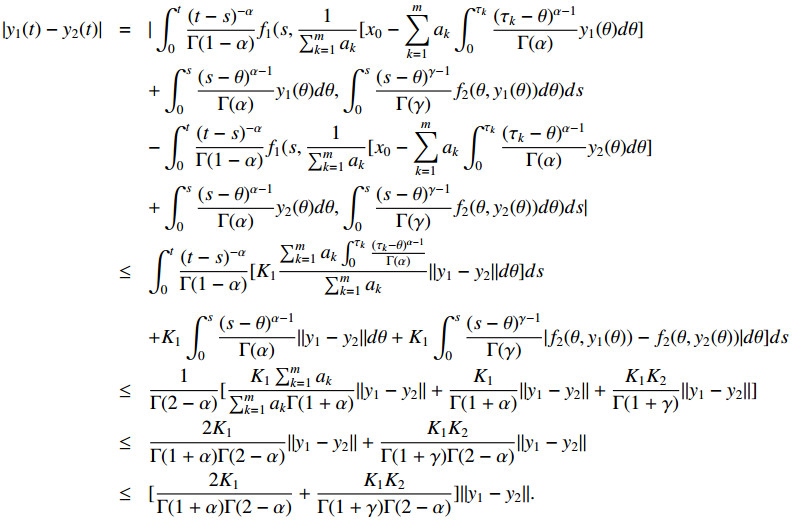
|
Then
| ‖y1−y2‖[αγΓ(2−α)−(2K1α+K1K2γ)]<0. |
Since (αγΓ(2−α)−(2K1α+K1K2γ))<1, then y1(t)=y2(t) and the solution of (1.2) and (2.1) is unique.
Definition 4.1. The unique solution of the problems (1.2) and (2.1) depends continuously on initial data x0, if ϵ>0, ∃δ>0, such that
| |x0−x∗0|≤δ⇒‖y−y∗‖≤ϵ, |
where y∗ is the unique solution of the integral equation
| y∗(t)=∫t0(t−s)−αΓ(1−α)f1(s,1∑mk=1ak[x∗0−m∑k=1ak∫τk0(τk−θ)α−1Γ(α)y∗(θ)dθ]+∫s0(s−θ)α−1Γ(α)y∗(θ)dθ,∫s0(s−θ)γ−1Γ(γ)f2(θ,y∗(θ))dθ)ds|. |
Theorem 4.2. Let the assumptions (I∗) and (II∗) be satisfied, then the unique solution of (1.2) and (2.1) depends continuously on x0.
Proof. Let y(t) and y∗(t) be the solutions of problems (1.2) and (2.1), then
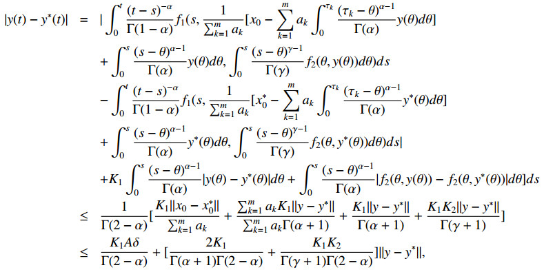
|
then we obtain
| |y(t)−y∗(t)|≤(AK1δ)(αγΓ(2−α)−(2K1α+K1K2γ))−1≤ϵ |
and
| ‖y(t)−y∗(t)‖≤ϵ. |
Definition 4.2. The unique solution of the problems (1.2) and (2.1) depends continuously on initial data ak, if ϵ>0, ∃δ>0, such that
| m∑k=1|ak−a∗k|≤δ⇒‖y−y∗‖≤ϵ, |
where y∗ is the unique solution of the integral equation
| y∗(t)=∫t0(t−s)−αΓ(1−α)f1(s,1∑mk=1ak[x0−m∑k=1a∗k∫τk0(τk−θ)α−1Γ(α)y∗(θ)dθ]+∫s0(s−θ)α−1Γ(α)y∗(θ)dθ,∫s0(s−θ)γ−1Γ(γ)f2(θ,y∗(θ))dθ)ds|. |
Theorem 4.3. Let the assumptions (I∗) and (II∗) be satisfied, then the unique solution of problems (1.2) and (2.1) depends continuously on ak.
Proof. Let y(t) and y∗(t) be the solutions of problems (1.2) and (2.1) and (∑mk=1a∗k)−1=A∗,
| |y(t)−y∗(t)|=|∫t0(t−s)−αΓ(1−α)f1(s,1∑mk=1ak[x0−m∑k=1ak∫τk0(τk−θ)α−1Γ(α)y(θ)dθ]+∫s0(s−θ)α−1Γ(α)y(θ)dθ,∫s0(s−θ)γ−1Γ(γ)f2(θ,y(θ))dθ)ds−∫t0(t−s)−αΓ(1−α)f1(s,1∑mk=1a∗k[x0−m∑k=1a∗k∫τk0(τk−θ)α−1Γ(α)y∗(θ)dθ]+∫s0(s−θ)α−1Γ(α)y∗(θ)dθ,∫s0(s−θ)γ−1Γ(γ)f2(θ,y∗(θ))dθ)ds|≤∫t0(t−s)−αΓ(1−α)[|x0|(∑mk=1a∗k−∑mk=1ak)∑mk=1ak∑mk=1a∗k+∑mk=1ak∫τk0(τk−θ)α−1Γ(α)|y(θ)|dθ∑mk=1ak−∑mk=1a∗k∫τk0(τk−θ)α−1Γ(α)|y∗(θ)|dθ∑mk=1a∗k+K1∫s0(s−θ)α−1Γ(α)|y(θ)−y∗(θ)|dθ+K1K2∫s0(s−θ)γ−1Γ(γ)|y(ϕ)−y∗(θ)|dθ]ds≤1Γ(2−α)[K1|x0|∑mk=1|a∗k−ak|∑mk=1ak∑mk=1a∗k+K1∑mk=1ak(∑mk=1a∗k∫τk0(τk−θ)α−1Γ(α)|y(θ)|dθ−∑mk=1ak∫τk0(τk−θ)α−1Γ(α)|y(θ)|dθ)∑mk=1ak∑mk=1a∗k+K1∑mk=1a∗k(∑mk=1ak∫τk0(τk−θ)α−1Γ(α)|y(θ)|dθ−∑mk=1a∗k∫τk0(τk−θ)α−1Γ(α)|y(θ)|dθ)∑mk=1ak∑mk=1a∗k+K1∫s0(s−θ)α−1Γ(α)|y(θ)−y∗(θ)|dθ+K1K2∫s0(s−θ)γ−1Γ(γ)|y(ϕ)−y∗(θ)|dθ]ds≤1Γ(2−α)[K1|x0|δ∑mk=1ak∑mk=1a∗k+K1(∑mk=1akδrΓ(α+1)+∑mk=1a∗kδrΓ(α+1))∑mk=1ak∑mk=1a∗k+K1‖y−y∗‖Γ(α+1)+K1K2‖y−y∗‖Γ(γ+1)≤K1δ|x0|Γ(2−α)∑mk=1ak∑mk=1a∗k+K1(∑mk=1akδrΓ(α+1)+∑mk=1a∗kδrΓ(α+1))Γ(2−α)Γ(α+1)∑mk=1ak∑mk=1a∗k+K1‖y−y∗‖Γ(2−α)Γ(α+1)+K1K2‖y−y∗‖Γ(γ+1)Γ(2−α), |
then we obtain
| \begin{eqnarray*} |y(t)-y^{*}(t)|\leq(AA^{*}K_{1}\delta [|x_{0}|+ r(\sum\limits^{m}_{k = 1}a_{k}+\sum\limits^{m}_{k = 1}a^{*}_{k})]).\; (\alpha\gamma\Gamma(2-\alpha)-(2K_{1}\alpha+K_{1}K_{2}\gamma))^{-1}\leq\epsilon \end{eqnarray*} |
and
| \begin{eqnarray*} &&\|y(t)-y^{*}(t)\|\leq\epsilon. \end{eqnarray*} |
Let y\in C[0, 1] be the solution of the nonlocal boundary value problems (1.2) and (2.1). Let a_{k} = (g(t_{k})-g(t_{k-1}) , g is increasing function, \tau_{k}\in(t_{k-1}-t_{k}) , 0 = t_{0} < t_{1} < t_{2}, ... < t_{m} = 1 , then, as m\longrightarrow \infty the nonlocal condition (1.2) will be
| \sum\limits^{m}_{k = 1}(g(t_{k})-g(t_{k-1})y(\tau_{k}) = x_{0}. |
As the limit m\longrightarrow \infty , we obtain
| \lim\limits_{m\rightarrow \infty}\sum\limits^{m}_{k = 1}(g(t_{k})-g(t_{k-1})y(\tau_{k}) = \int_{0}^{1}y(s)dg(s) = x_{0}. |
Theorem 5.1. Let the assumptions (I)–(III) be satisfied. If \sum\nolimits^{m}_{k = 1}a_{k} be convergent, then the nonlocal boundary value problems of (1.3) and (2.1) have at least one solution given by
| \begin{eqnarray*} y(t)& = &\int_{0}^{t}\frac{(t-s)^{-\alpha}}{\Gamma(1-\alpha)} f_{1}(s,\frac{1}{g(1)-g(0)}[x_{0}-\int_{0}^{1}\int_{0}^{s}\frac{(s-\theta)^{\alpha-1}}{\Gamma(\alpha)}y(\theta)d\theta dg(s)]\\ &&+\int_{0}^{s}\frac{(s-\theta)^{\alpha-1}}{\Gamma(\alpha)}y(\theta)d\theta,\int_{0}^{s}\frac{(s-\theta)^{\gamma-1}}{\Gamma(\gamma)}f_{2} (\phi,y(\theta))d\theta)ds. \end{eqnarray*} |
Proof. As m\rightarrow \infty , the solution of the nonlocal boundary value problem (2.1) will be
| \begin{eqnarray*} \lim\limits_{m\rightarrow \infty}y(t)& = &\int_{0}^{t}\frac{(t-s)^{-\alpha}}{\Gamma(1-\alpha)} f_{1}(s,(g(1)-g(0))^{-1}x_{0}\\ &&-(g(1)-g(0))^{-1}.\lim\limits_{m\rightarrow \infty}\sum\limits^{m}_{k = 1}[g(t_{k})-g(t_{k-1}]\int_{0}^{\tau_{k}}\frac{(\tau_{k}-\theta)^{\alpha-1}}{\Gamma(\alpha)}y(\theta)d\theta\\ &&+\int_{0}^{s}\frac{(s-\theta)^{\alpha-1}}{\Gamma(\alpha)}y(\theta)d\theta,\int_{0}^{s}\frac{(s-\theta)^{\gamma-1}}{\Gamma(\gamma)} f_{2}(\phi,y(\theta))d\theta)ds\\ & = &\int_{0}^{t}\frac{(t-s)^{-\alpha}}{\Gamma(1-\alpha)} f_{1}(s,\frac{1}{g(1)-g(0)}[x_{0}-\int_{0}^{1}\int_{0}^{s}\frac{(s-\theta)^{\alpha-1}}{\Gamma(\alpha)}y(\theta)d\theta dg(s)]\\ &&+\int_{0}^{s}\frac{(s-\theta)^{\alpha-1}}{\Gamma(\alpha)}y(\theta)d\theta,\int_{0}^{s}\frac{(s-\theta)^{\gamma-1}}{\Gamma(\gamma)} f_{2}(\phi,y(\theta))d\theta)ds. \end{eqnarray*} |
Theorem 6.1. Let the assumptions (I)–(III) be satisfied, then the nonlocal boundary value problems of (1.4) and (2.1) have at least one solution given by
| \begin{eqnarray} y(t)& = &\int_{0}^{t}\frac{(t-s)^{-\alpha}}{\Gamma(1-\alpha)} f_{1}(s,\frac{1}{\sum\nolimits^{\infty}_{k = 1}a_{k}}[x_{0}-\sum\limits^{\infty}_{k = 1}a_{k}\int_{0}^{\tau_{k}}\frac{(\tau_{k}-\theta)^{\alpha-1}} {\Gamma(\alpha)}y(\theta)d\theta]\\ &&+\int_{0}^{s}\frac{(s-\theta)^{\alpha-1}}{\Gamma(\alpha)}y(\theta)d\theta,\int_{0}^{s}\frac{(s-\theta)^{\gamma-1}}{\Gamma(\gamma)} f_{2}(\phi,y(\theta))d\theta)ds. \end{eqnarray} |
Proof. Let the assumptions of Theorem 2.1 be satisfied. Let \sum\nolimits^{m}_{k = 1} a_{k} be convergent, then take the limit to (1.4), we have
| \begin{eqnarray} \lim\limits_{m\rightarrow \infty}y(t)& = &\int_{0}^{t}\frac{(t-s)^{-\alpha}}{\Gamma(1-\alpha)} f_{1}(s,\lim\limits_{m\rightarrow m}\frac{1}{\sum\nolimits^{m}_{k = 1}a_{k}}[x_{0}-\lim\limits_{m\rightarrow \infty}\sum\limits^{m}_{k = 1}a_{k}\int_{0}^{\tau_{k}}\frac{(\tau_{k}-\theta)^{\alpha-1}}{\Gamma(\alpha)}y(\theta)d\theta]\\ &&+\int_{0}^{s}\frac{(s-\theta)^{\alpha-1}}{\Gamma(\alpha)}y(\theta)d\theta,\int_{0}^{s}\frac{(s-\theta)^{\gamma-1}}{\Gamma(\gamma)}f_{2}(\phi,y(\theta))d\theta)ds. \end{eqnarray} |
Now
| \begin{eqnarray*} |a_{k}\int_{0}^{\tau_{k}}\frac{(\tau_{k}-\theta)^{\alpha-1}}{\Gamma(\alpha)}y(\theta)d\theta| \leq|a_{k}|\int_{0}^{\tau_{k}}\frac{(\tau_{k}-\theta)^{\alpha-1}}{\Gamma(\alpha)}|y(\theta)|d\theta\leq\frac{|a_{k}|\|y\|}{\Gamma(\alpha+1)} \leq\frac{|a_{k}|r}{\Gamma(\alpha+1)} \end{eqnarray*} |
and by the comparison test (\sum\nolimits^{m}_{k = 1}a_{k}\int_{0}^{\tau_{k}}\frac{(\tau_{k}-\theta)^{\alpha-1}}{\Gamma(\alpha)}y(\theta)d\theta) is convergent,
| \begin{eqnarray*} y(t)& = &\int_{0}^{t}\frac{(t-s)^{-\alpha}}{\Gamma(1-\alpha)} f_{1}(s,\frac{1}{\sum\nolimits^{\infty}_{k = 1}a_{k}}[x_{0}-\sum\limits^{\infty}_{k = 1}a_{k}\int_{0}^{\tau_{k}}\frac{(\tau_{k}-\theta)^{\alpha-1}}{\Gamma(\alpha)}y(\theta)d\theta]\nonumber\\ &&+\int_{0}^{s}\frac{(s-\theta)^{\alpha-1}}{\Gamma(\alpha)}y(\theta)d\theta,\int_{0}^{s}\frac{(s-\theta)^{\gamma-1}}{\Gamma(\gamma)}f_{2}(\phi,y(\theta))d\theta)ds.\nonumber \end{eqnarray*} |
Furthermore, from (2.9) we have
| \begin{eqnarray*} \sum\limits^{\infty}_{k = 1}a_{k}x(\tau_{k})& = &\sum\limits^{\infty}_{k = 1}a_{k}[\frac{1}{\sum\nolimits^{\infty}_{k = 1}a_{k}}(x_{0}-\sum\limits^{\infty}_{k = 1}a_{k}\int_{0}^{\tau_{k}}\frac{(\tau_{k}-s)^{\alpha-1}}{\Gamma(\alpha)}y(s)ds)]\\ &&+\int_{0}^{\tau_{k}}\frac{(\tau_{k}-s)^{\alpha-1}}{\Gamma(\alpha)}y(s)ds)]\\ & = &x_{0}. \end{eqnarray*} |
Example 6.1. Consider the following nonlinear integro-differential equation
| \begin{equation} \frac{dx}{dt} = t^{4}e^{-t}+\frac{x(t)}{\sqrt{t+2}}+\frac{1}{3}I^{\gamma}(\cos(5t+1)+\frac{1}{9}[t^{5}\sin D^{\frac{1}{3}}x(t)+e^{-3t}x(t)]) \end{equation} | (6.1) |
with boundary condition
| \begin{equation} {\sum\limits^{m}_{k = 1}\bigg[\frac{1}{k}-\frac{1}{k+1}\bigg]} x(\tau_k ) = x_{0},\; a_{k} > 0\; \; \tau_{k}\in[0,1]. \end{equation} | (6.2) |
Let
| \begin{eqnarray*} f_{1}(t,x(t),I^{\gamma}f_{2}(t,D^{\alpha}x(t))) = t^{4}e^{-t}+\frac{x(t)}{\sqrt{t+2}}+\frac{1}{3}I^{\gamma}(\cos(5t+1)+\frac{1}{9}[t^{5}\sin D^{\frac{1}{3}}x(t)+e^{-3t}x(t)]), \end{eqnarray*} |
then
| \begin{eqnarray*} |f_{1}(t,x(t),I^{\gamma}f_{2}(t,D^{\alpha}x(t))) = |t^{4}e^{-t}+\frac{x(t)}{\sqrt{2t+4}}+\\ \frac{1}{4}(\frac{4}{3}I^{\gamma}(\cos(5t+1)+\frac{1}{9}[t^{5}\sin D^{\frac{1}{3}}x(t)+e^{-3t}x(t)]))| \end{eqnarray*} |
and also
| \begin{eqnarray*} &&|I^{\gamma}f_{2}(t,D^{\alpha}x(t))|\leq \frac{1}{4}(\frac{4}{3}I^{\gamma}|\cos(5t+1)+\frac{1}{3}[t^{5}\sin D^{\frac{1}{3}}x(t)+e^{-3t}x(t)]|. \end{eqnarray*} |
It is clear that the assumptions (I) and (II) of Theorem 2.1 are satisfied with a_{1}(t) = t^{4}e^{-t}\in L^{1}[0, 1] , a_{2}(t) = \frac{4}{3}I^{\gamma}|(\cos(5t+1)|\in L^{1}[0, 1] , and let \alpha = \frac{1}{3} , \gamma = \frac{2}{3} , then 2K_{1}\gamma+K_{1}K_{2}\alpha = \frac{1}{2} < \alpha\gamma\Gamma(2-\alpha) = \frac{1}{2}\Gamma(2-\alpha) . Therefore, by applying Theorem 2.1, the nonlocal problems (6.1) and (6.2) has a continuous solution.
In this paper, we have studied a boundary value problem of fractional order differential inclusion with nonlocal, integral and infinite points boundary conditions. We have prove some existence results for that a single nonlocal boundary value problem, in of proving some existence results for a boundary value problem of fractional order differential inclusion with nonlocal, integral and infinite points boundary conditions. Next, we have proved the existence of maximal and minimal solutions. Then we have established the sufficient conditions for the uniqueness of solutions and continuous dependence of solution on some initial data and on the coefficients a_k are studied. Finally, we have proved the existence of a nonlocal boundary value problem with Riemann-Stieltjes integral condition and with infinite-point boundary condition. An example is given to illustrate our results.
The authors declare no conflict of interest.
| [1] |
S. Banach, Sur les operations dans les ensembles abstraits et leur application aux equations integrales, Fund. Math., 3 (1922), 133–181. https://doi.org/10.4064/fm-3-1-133-181 doi: 10.4064/fm-3-1-133-181

|
| [2] | E. Picard, Memoire sur la theorie des equations aux derivees partielles et la methode des approximations successives, J. Math. Pures Appl., 6 (1880), 145–210. http://www.numdam.org/item/?id = JMPA_1890_4_6__145_0 |
| [3] |
F. E. Browder, Nonexpansive nonlinear operators in a Banach space, Proc. Natl. Acad. Sci., 54 (1965), 1041–1044. https://doi.org/10.1073/pnas.54.4.1041 doi: 10.1073/pnas.54.4.1041
|
| [4] |
D. Gohde, Zum Prinzip der Kontraktiven Abbildung, Math. Nachr., 30 (1965), 251–258. https://doi.org/10.1002/mana.19650300312 doi: 10.1002/mana.19650300312
|
| [5] |
W. A. Kirk, A fixed point theorem for mappings which do not increase distance, Am. Math. Mon., 72 (1965), 1004–1006. https://doi.org/10.2307/2313345 doi: 10.2307/2313345
|
| [6] |
T. Suzuki, Fixed point theorems and convergence theorems for some generalized non-expansive mapping, J. Math. Anal. Appl., 340 (2008), 1088–1095. https://doi.org/10.1016/j.jmaa.2007.09.023 doi: 10.1016/j.jmaa.2007.09.023
|
| [7] |
B. S. Thakur, D. Thakur, M. Postolache, A new iterative scheme for numerical reckoning fixed points of Suzuki's generalized nonexpansive mappings, Appl. Math. Comput., 225 (2016), 147–155. https://doi.org/10.1016/j.amc.2015.11.065 doi: 10.1016/j.amc.2015.11.065
|
| [8] |
K. Ullah, M. Arshad, Numerical reckoning fixed points for Suzuki's generalized nonexpansive mappings via new iteration process, Filomat, 32 (2018), 187–196. https://doi.org/10.2298/FIL1801187U doi: 10.2298/FIL1801187U
|
| [9] | E. Karapinar, K. Tas, Generalized (C)–conditions and related fixed point theorems, Comput. Math. Appl., 61 (2011), 3370–3380. |
| [10] |
Y. Jia, M. Xu, Y. Lin, D. Jiang, An efficient technique based on least-squares method for fractional integro-differential equations, Alex. Eng. J., 64 (2023), 97–105. https://doi.org/10.1016/j.aej.2022.08.033 doi: 10.1016/j.aej.2022.08.033
|
| [11] |
W. R. Mann, Mean value methods in iteration, Proc. Amer. Math. Soc., 4 (1953), 506–510. https://doi.org/10.1090/S0002-9939-1953-0054846-3 doi: 10.1090/S0002-9939-1953-0054846-3
|
| [12] |
S. Ishikawa, Fixed points by a new iteration method, Proc. Amer. Math. Soc., 44 (1974), 147–150. https://doi.org/10.1090/S0002-9939-1974-0336469-5 doi: 10.1090/S0002-9939-1974-0336469-5
|
| [13] |
M. A. Noor, New approximation schemes for general variational inequalities, J. Math. Anal. Appl., 251 (2000), 217–229. https://doi.org/10.1006/jmaa.2000.7042 doi: 10.1006/jmaa.2000.7042
|
| [14] | R. P. Agarwal, D. O'Regon, D. R. Sahu, Iterative construction of fixed points of nearly asymptotically nonexpansive mappings, J. Nonlinear Convex Anal., 8 (2007), 61–79. |
| [15] | M. Abbas, T. Nazir, A new faster iteration process applied to constrained minimization and feasibility problems, Mat. Vestn., 66 (2014), 223–234. |
| [16] |
N. Wairojjana, N. Pakkaranang, N. Pholasa, Strong convergence inertial projection algorithm with self-adaptive step size rule for pseudomonotone variational inequalities in Hilbert spaces, Demonstratio Math., 54, (2021), 110–128. https://doi.org/10.1515/dema-2021-0011 doi: 10.1515/dema-2021-0011
|
| [17] | S. Khatoon, I. Uddin, Convergence analysis of modified Abbas iteration process for two G-nonexpansive mappings, Rendiconti del Circolo Matematico di Palermo Series, 2 (2021), 31–44. |
| [18] |
H. A. Hammad, H. U. Rehman, M. Zayed, Applying faster algorithm for obtaining convergence, stability, and data dependence results with application to functional-integral equations, AIMS Math., 7 (2020), 19026–19056. https://doi.org/10.3934/math.20221046 doi: 10.3934/math.20221046
|
| [19] | H. A. Hammad, H. U. Rehman, M. De la Sen, M. A novel four-step iterative scheme for approximating the fixed point with a supportive application, Inf. Sci. Lett., 10 (2021), 14. |
| [20] | H. A. Hammad, H. U. Rehman, M. De la Sen, Shrinking projection methods for accelerating relaxed inertial Tseng-type algorithm with applications, Math. Prob. Eng., 2020 (2020), Article ID 7487383, 14 pages. https://doi.org/10.1155/2020/7487383 |
| [21] |
J. A. Clarkson, Uniformly convex spaces, Trans. Amer. Math. Soc., 40 (1936), 396–414. https://doi.org/10.1090/S0002-9947-1936-1501880-4 doi: 10.1155/2020/7487383
|
| [22] | R. P. Agarwal, D. O'Regan, D. R. Sahu, Fixed Point Theory for Lipschitzian-Type Mappings with Applications Series, New York: Springer, (2009). |
| [23] | W. Takahashi, Nonlinear Functional Analysis, Yokohoma: Yokohoma Publishers, (2000). |
| [24] |
Z. Opial, Weak convergence of the sequence of successive approximations for nonexpansive mappings, Bull. Amer. Math. Soc., 73 (1967), 591–597. https://doi.org/10.1090/S0002-9904-1967-11761-0 doi: 10.1090/S0002-9904-1967-11761-0
|
| [25] |
H. F. Senter, W. G. Dotson, Approximating fixed points of nonexpansive mappings, Proc. Amer. Math. Soc., 44 (1974), 375–380. https://doi.org/10.1090/S0002-9939-1974-0346608-8 doi: 10.1090/S0002-9939-1974-0346608-8
|
| [26] |
J. Schu, Weak and strong convergence to fixed points of asymptotically nonexpansive mappings, Bull. Aust. Math. Soc., 43 (1991), 153–159. https://doi.org/10.1017/S0004972700028884 doi: 10.1017/S0004972700028884
|
| [27] |
J. Ali, M. Jubair, F. Ali, Stability and convergence of F iterative scheme with an application tot the fractional differential equation, Eng. Comput., 38 (2022), 693–702. https://doi.org/10.1007/s00366-020-01172-y doi: 10.1007/s00366-020-01172-y
|
| [28] | E. Karapnar, T. Abdeljawad, F. Jarad, Applying new fixed point theorems on fractional and ordinary differential equations, Adv. Differ. Eq. 421 (2019), 1–25. |
| [29] | S. Khatoon, I. Uddin, D. Beleanu, Approximation of fixed point and its application to fractional differential equation, J. Appl. Math. Comput., 2020 (2020), 1–20. |
| [30] |
H. A. Hammad, H. U. Rehman, M. De la Sen, A New four-step iterative procedure for approximating fixed points with application to 2D Volterra integral equations, Mathematics, 10 (2022), 4257. https://doi.org/10.3390/math10224257 doi: 10.3390/math10224257
|
| [31] |
H. A. Hammad, P. Agarwal, S. Momani, F. Alsharari, Solving a fractional-order differential equation using rational symmetric contraction mappings, Fractal Fract., 5 (2021), 159. https://doi.org/10.3390/fractalfract5040159 doi: 10.3390/fractalfract5040159
|
| [32] |
H. A. Hammad, M. Zayed, Solving a system of differential equations with infinite delay by using tripled fixed point techniques on graphs, Symmetry, 14 (2022), 1388. https://doi.org/10.3390/sym14071388 doi: 10.3390/sym14071388
|

Figures(1) / Tables(2)

Junaid Ahmad, Kifayat Ullah, Hasanen A. Hammad, Reny George. A solution of a fractional differential equation via novel fixed-point approaches in Banach spaces[J]. AIMS Mathematics, 2023, 8(6): 12657-12670. doi: 10.3934/math.2023636


 DownLoad: