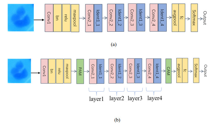
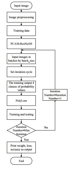
Somatic cell count (SCC) is a fundamental approach for determining the quality of cattle and bovine milk. So far, different classification and recognition methods have been proposed, all with certain limitations. In this study, we introduced a new deep learning tool, i.e., an improved ResNet50 model constructed based on the residual network and fused with the position attention module and channel attention module to extract the feature information more effectively. In this paper, macrophages, lymphocytes, epithelial cells, and neutrophils were assessed. An image dataset for milk somatic cells was constructed by preprocessing to increase the diversity of samples. PolyLoss was selected as the loss function to solve the unbalanced category samples and difficult sample mining. The Adam optimization algorithm was used to update the gradient, while Warm-up was used to warm up the learning rate to alleviate the overfitting caused by small sample data sets and improve the model's generalization ability. The experimental results showed that the classification accuracy, precision rate, recall rate, and comprehensive evaluation index F value of the proposed model reached 97%, 94.5%, 90.75%, and 92.25%, respectively, indicating that the proposed model could effectively classify the milk somatic cell images, showing a better classification performance than five previous models (i.e., ResNet50, ResNet18, ResNet34, AlexNet andMobileNetv2). The accuracies of the ResNet18, ResNet34, ResNet50, AlexNet, MobileNetv2, and the new model were 95%, 93%, 93%, 56%, 37%, and 97%, respectively. In addition, the comprehensive evaluation index F1 showed the best effect, fully verifying the effectiveness of the proposed method in this paper. The proposed method overcame the limitations of image preprocessing and manual feature extraction by traditional machine learning methods and the limitations of manual feature selection, improving the classification accuracy and showing a strong generalization ability.
Citation: Jie Bai, Heru Xue, Xinhua Jiang, Yanqing Zhou. Classification and recognition of milk somatic cell images based on PolyLoss and PCAM-Reset50[J]. Mathematical Biosciences and Engineering, 2023, 20(5): 9423-9442. doi: 10.3934/mbe.2023414
Somatic cell count (SCC) is a fundamental approach for determining the quality of cattle and bovine milk. So far, different classification and recognition methods have been proposed, all with certain limitations. In this study, we introduced a new deep learning tool, i.e., an improved ResNet50 model constructed based on the residual network and fused with the position attention module and channel attention module to extract the feature information more effectively. In this paper, macrophages, lymphocytes, epithelial cells, and neutrophils were assessed. An image dataset for milk somatic cells was constructed by preprocessing to increase the diversity of samples. PolyLoss was selected as the loss function to solve the unbalanced category samples and difficult sample mining. The Adam optimization algorithm was used to update the gradient, while Warm-up was used to warm up the learning rate to alleviate the overfitting caused by small sample data sets and improve the model's generalization ability. The experimental results showed that the classification accuracy, precision rate, recall rate, and comprehensive evaluation index F value of the proposed model reached 97%, 94.5%, 90.75%, and 92.25%, respectively, indicating that the proposed model could effectively classify the milk somatic cell images, showing a better classification performance than five previous models (i.e., ResNet50, ResNet18, ResNet34, AlexNet andMobileNetv2). The accuracies of the ResNet18, ResNet34, ResNet50, AlexNet, MobileNetv2, and the new model were 95%, 93%, 93%, 56%, 37%, and 97%, respectively. In addition, the comprehensive evaluation index F1 showed the best effect, fully verifying the effectiveness of the proposed method in this paper. The proposed method overcame the limitations of image preprocessing and manual feature extraction by traditional machine learning methods and the limitations of manual feature selection, improving the classification accuracy and showing a strong generalization ability.

| [1] |
T. Halasa, K. Huijps, O. Østerås, H. Hogeveen, Economic effects of bovine mastitis and mastitis management: a review, Vet. Q., 29 (2007), 18–31. https://doi.org/10.1080/01652176.2007.9695224 doi: 10.1080/01652176.2007.9695224

|
| [2] |
U. Geary, N. Lopez-Villalobos, N. Begley, F. Mccoy, B. O. Brien, L. O. Grady, Estimating the effect of mastitis on the profitability of irish dairy farms, J. Dairy Sci., 95 (2012), 3662–3673. https://doi.org/10.3168/jds.2011-4863 doi: 10.3168/jds.2011-4863
|
| [3] | D. Barrett, High somatic cell counts-a persistent problem, Irish Vet. J., 55 (2002), 173–178. |
| [4] |
H. M. Golder, A. Hodge, I. J. Lean, Effects of antibiotic dry-cow therapy and internal teat sealant on milk somatic cell counts and clinical and subclinical mastitis in early lactation, J. Dairy Sci., 99 (2016), 7370–7380. https://doi.org/10.3168/jds.2016-11114 doi: 10.3168/jds.2016-11114
|
| [5] | J. Hamann, Changes in milk somatic cell count with regard to the milking process and the milking frequen, Bull. Int. Dairy Fed., 24 (2001), 5–6. |
| [6] |
G. Leitner, Y. Lavon, Z. Matzrafi, O. Benun, D. Bezman, U. Merin, Somatic cell counts, chemical composition and coagulation properties of goat and sheep bulk tank milk, Int. Dairy J., 58 (2016), 9–13. https://doi.org/10.1016/j.idairyj.2015.11.004 doi: 10.1016/j.idairyj.2015.11.004
|
| [7] |
U. K. Sundekilde, N. A. Poulsen, L. B. Larsen, H. C. Bertram, Nuclear magnetic resonance metabonomics reveals strong association between milk metabolites and somatic cell count in bovine milk, J. Dairy Sci., 96 (2013), 290–299. https://doi.org/10.3168/jds.2012-5819 doi: 10.3168/jds.2012-5819
|
| [8] |
J. S. Moon, H. C. Koo, Y. S. Joo, S. H. Jeon, D. S. Hur, C. I. Chung, Application of a new portable microscopic somatic cell counter with disposable plastic chip for milk analysis, J. Dairy Sci., 90 (2007), 2253–2259. https://doi.org/10.3168/jds.2006-622 doi: 10.3168/jds.2006-622
|
| [9] | A. Awad, and M. Hassaballah, Image Feature Detectors and Descriptors, Springer, (2016). |
| [10] |
S. U. Khan, N. Islam, Z. Jan, K. Haseeb, S. I. A. Shah, M. Hanif, A machine learning-based approach for the segmentation and classification of malignant cells in breast cytology images using gray level co-occurrence matrix (GLCM) and support vector machine (SVM), Neural Comput. Appl., 34 (2022), 8365–8372. https://doi.org/10.1007/s00521-021-05697-1 doi: 10.1007/s00521-021-05697-1
|
| [11] |
H. B. ökmen, A. Guvenis, H. Uysal, Predicting the polybromo-1 (PBRM1) mutation of a clear cell renal cell carcinoma using computed tomography images and knn classification with random subspace, Vibroeng. Procedia, 26 (2019), 30–34. https://doi.org/10.21595/vp.2019.20931 doi: 10.21595/vp.2019.20931
|
| [12] |
S. Mishra, B. Majhi, P. K. Sa, L. Sharma, Gray level co-occurrence matrix and random forest based acute lymphoblastic leukemia detection, Biomed. Signal Process. Control, 33 (2017), 272–280. https://doi.org/10.1016/j.bspc.2016.11.021 doi: 10.1016/j.bspc.2016.11.021
|
| [13] |
X. J. Gao, H. R. Xue, X. Pan, X. H. Jiang, Y. Q. Zhou, X. L. Luo, Somatic cells recognition by application of Gabor feature-based (2D)2PCA, Int. J. Pattern Recognit Artif. Intell., 31 (2017), 1757009. https://doi.org/10.1142/S0218001417570099 doi: 10.1142/S0218001417570099
|
| [14] |
X. J. Gao, H. R. Xue, X. Pan, X. L. Luo, Polymorphous bovine somatic cell recognition based on feature fusion, Int. J. Pattern Recognit Artif. Intell., 34 (2020), 2050032. https://doi.org/10.1142/S0218001420500329 doi: 10.1142/S0218001420500329
|
| [15] |
X. J. Gao, H. R. Xue, X. H. Jiang, Y. Q. Zhou, Recognition of somatic cells in bovine milk using fusion feature, Int. J. Pattern Recognit Artif. Intell., 32 (2018), 1850021. https://doi.org/10.1142/S0218001418500210 doi: 10.1142/S0218001418500210
|
| [16] |
X. L. Zhang, H. R. Xue, X. J. Gao, Y. Q. Zhou, Milk somatic cells recognition based on multi-feature fusion and random forest, J. Inn. Mongolia Agric. Univ., 39 (2018), 87–92. https://doi.org/10.16853/j.cnki.1009-3575.2018.06.014 doi: 10.16853/j.cnki.1009-3575.2018.06.014
|
| [17] |
J. Zhang, C. Li, M. M. Rahaman, Y. Yao, P. Ma, J. Zhang, et al., A comprehensive survey with quantitative comparison of image analysis methods for microorganism biovolume measurements, Arch. Comput. Methods Eng., 30 (2023), 639–673. https://doi.org/10.1007/s11831-022-09811-x doi: 10.1007/s11831-022-09811-x
|
| [18] |
P. Ma, C. Li, M. Rahaman, Y. Yao, J. Zhang, S. Zou, et al., A state-of-the-art survey of object detection techniques in microorganism image analysis: from classical methods to deep learning approaches, Artif. Intell. Rev., 56 (2023), 1627–1698. https://doi.org/10.1007/s10462-022-10209-1 doi: 10.1007/s10462-022-10209-1
|
| [19] |
J. Zhang, C. Li, Y. Yin, J. Zhang, M. Grzegorzek, Applications of artificial neural networks in microorganism image analysis: a comprehensive review from conventional multilayer perceptron to popular convolutional neural network and potential visual transformer, Artif. Intell. Rev., 56 (2023), 1013–1070. https://doi.org/10.1007/s10462-022-10192-7 doi: 10.1007/s10462-022-10192-7
|
| [20] |
J. Zhang, C. Li, M. M. Rahaman, Y. Yao, P. Ma, J. Zhang, et al., A comprehensive review of image analysis methods for microorganism counting: from classical image processing to deep learning approaches, Artif. Intell. Rev., 55 (2022), 2875–2944. https://doi.org/10.1007/s10462-021-10082-4 doi: 10.1007/s10462-021-10082-4
|
| [21] |
G. Liang, H. Hong, W. Xie, L. Zheng, Combining convolutional neural network with recursive neural network for blood cell image classification, IEEE Access, 6 (2018), 36188–36197. https://doi.org/10.1109/ACCESS.2018.2846685 doi: 10.1109/ACCESS.2018.2846685
|
| [22] | D. Bani-Hani, N. Khan, F. Alsultan, S. Karanjkar, N. Nagarur, Classification of leucocytes using convolutional neural network optimized through genetic algorithm, in Proceedings of the 7th Annual World Conference of the Society for Industrial and Systems Engineering, (2018), 1–6. |
| [23] | M. Habibzadeh, M. Jannesari, Z. Rezaei, H. Baharvand, M. Totonchi, Automatic white blood cell classification using pre-trained deep learning models: resnet and inception, in 10th International Conference on Machine Vision (ICMV 2017), (2018), 274–281. https://doi.org/10.1117/12.2311282 |
| [24] |
A. Acevedo, S. Alférez, A. Merino, L. Puigví, J. Rodellar, Recognition of peripheral blood cell images using convolutional neural networks, Comput. Methods Programs Biomed., 180 (2019), 105020. https://doi.org/10.1016/j.cmpb.2019.105020 doi: 10.1016/j.cmpb.2019.105020
|
| [25] | A. Malkawi, R. Al-Assi, T. Salameh, H. Alquran, A. M. Alqudah, White blood cells classification using convolutional neural network hybrid system, in 2020 IEEE 5th Middle East and Africa Conference on Biomedical Engineering (MECBME), (2020), 1–5. https://doi.org/10.1109/MECBME47393.2020.9265154 |
| [26] | I. Ghosh, S. Kundu, Combining neural network models for blood cell classification, arXiv preprint, 2021, arXiv: 2101.03604. https://doi.org/10.48550/arXiv.2101.03604 |
| [27] |
O. Russakovsky, J. Deng, H. Su, J. Krause, S. Satheesh, S. Ma, et al., Imagenet large scale visual recognition challenge, Int. J. Comput. Vision, 115 (2015), 211–252. https://doi.org/10.1007/s11263-015-0816-y doi: 10.1007/s11263-015-0816-y
|
| [28] | M. Sandler, A. Howard, M. Zhu, A. Zhmoginov, L. Chen, Mobilenetv2: in-verted residuals and linear bottlenecks, in 2018 IEEE/CVF Conference on Computer Vision and Pattern Recognition, (2018), 4510–4520. https://doi.org/10.1109/CVPR.2018.00474 |
| [29] |
Y. Hu, D. Y. Luo, K. Hua, H. M. Lu, X. G. Zhang, Overview on deep learning, CAAI Trans. Intell. Syst., 14 (2019), 1–19. https://doi.org/10.11992/tis.201808019 doi: 10.11992/tis.201808019
|
| [30] | A. I. Awad, M. Hassaballah, Deep Learning in Computer Vision, CRC Press, 2021. |
| [31] | K. He, X. Zhang, S. Ren, J. Sun, Deep residual learning for image recognition, in 2016 IEEE Conference on Computer Vision and Pattern Recognition (CVPR), (2016), 770–778. https://doi.org/10.1109/CVPR.2016.90 |
| [32] | X. J. Gao, Research of Polymorphous Bovine Somatic Cell Recognition Based on Feature Fusion, Ph.D thesis, Inner Mongolia Agricultural University in Huhhot, 2018. |
| [33] |
Y. Li, S. Tong, T. Li, Composite adaptive fuzzy output feedback control design for uncertain nonlinear strict-feedback systems with input saturation, IEEE Trans. Cybern., 45 (2015), 2299–2308. https://doi.org/10.1109/TCYB.2014.2370645 doi: 10.1109/TCYB.2014.2370645
|
| [34] |
Z. F. Jiang, T. He, Y. L. Shi, X. Long, S. H. Yang, Remote sensing image classification based on convolutional block attention module and deep residual network, Laser J., 43 (2022), 76–81. https://doi.org/10.14016/j.cnki.jgzz.2022.04.076 doi: 10.14016/j.cnki.jgzz.2022.04.076
|
| [35] | J. Fu, J. Liu, H. J. Tian, Y. Li, Y. J. Bao, Z. W. Fang, et al., Dual attention network for scene segmentation, in 2019 IEEE/CVF Conference on Computer Vision and Pattern Recognition (CVPR), (2019), 3141–3149. https://doi.org/10.1109/CVPR.2019.00326 |
| [36] | T. Lin, P. Goyal, R. Girshick, K. He, P. Dollar, Focal loss for dense object detection, in 2017 IEEE International Conference on Computer Vision (ICCV), (2017), 2999–3007. https://doi.org/10.1109/ICCV.2017.324 |
| [37] | Z. Q. Leng, M. X. Tan, C. X. Liu, E. D. Cubuk, X. J. Shi, S. Y. Cheng, et al., Polyloss: a polynomial expansion perspective of classification loss functions, arXiv preprint, arXiv: 2204.12511. https://doi.org/10.48550/arXiv.2204.12511 |
| [38] |
J. Bai, H. R. Xue, X. H. Jiang, Y. Q. Zhou, Recognition of bovine milk somatic cells based on multi-feature extraction and a gbdt-adaboost fusion model, Math. Biosci. Eng., 19 (2022), 5850–5866. https://doi.org/10.3934/mbe.2022274 doi: 10.3934/mbe.2022274
|
| [39] | D. P. Kingma, J. Ba, Adam: a method for stochastic optimization, arXiv preprint, arXiv: 1412.6980. https://doi.org/10.48550/arXiv.1412.6980 |
| [40] |
J. Zhang, C. Li, S. Kosov, M. Grzegorzek, K. Shirahama, T. Jiang, et al., LCU-Net: A novel low-cost U-Net for environmental microorganism image segmentation, Pattern Recognit., 115 (2021), 107885. https://doi.org/10.1016/j.patcog.2021.107885 doi: 10.1016/j.patcog.2021.107885
|
| [41] |
H. Chen, C. Li, X. Li, M. M. Rahaman, W. Hu, Y. Li, et al., IL-MCAM: An interactive learning and multi-channel attention mechanism-based weakly supervised colorectal histopathology image classification approach, Comput. Biol. Med., 143 (2022), 105265. https://doi.org/10.1016/j.compbiomed.2022.105265 doi: 10.1016/j.compbiomed.2022.105265
|
| [42] |
X. Li, C. Li, M. M. Rahaman, H. Sun, X. Li, J. Z. Wu, et al., A comprehensive review of computer-aided whole-slide image analysis: from datasets to feature extraction, segmentation, classification and detection approaches, Artif. Intell. Rev., 35 (2022), 4809–4878. https://doi.org/10.1007/s10462-021-10121-0 doi: 10.1007/s10462-021-10121-0
|
| [43] |
F. Kulwa, C. Li, J. Zhang, K. Shirahama, S. Kosov, X. Zhao, et al., A new pairwise deep learning feature for environmental microorganism image analysis, Environ. Sci. Pollut. Res., 29 (2022), 51909–51926. https://doi.org/10.1007/s11356-022-18849-0 doi: 10.1007/s11356-022-18849-0
|
| [44] |
A. Chen, C. Li, S. Zou, M. M. Rahaman, Y. Yao, H. Chen, et al., SVIA dataset: A new dataset of microscopic videos and images for computer-aided sperm analysis, Biocybern. Biomed. Eng., 42 (2022), 204–214. https://doi.org/10.1016/j.bbe.2021.12.010 doi: 10.1016/j.bbe.2021.12.010
|
Figures(12) / Tables(7)

Jie Bai, Heru Xue, Xinhua Jiang, Yanqing Zhou. Classification and recognition of milk somatic cell images based on PolyLoss and PCAM-Reset50[J]. Mathematical Biosciences and Engineering, 2023, 20(5): 9423-9442. doi: 10.3934/mbe.2023414


 DownLoad: