Big data analysis of water quality monitoring results from the Xiang River and an impact analysis of pollution management policies

Yangyan Zeng; Yidong Zhou; Wenzhi Cao; Dongbin Hu; Yueping Luo; Haiting Pan; Yangyan Zeng; Yidong Zhou; Wenzhi Cao; Dongbin Hu; Yueping Luo; Haiting Pan

doi:10.3934/mbe.2023415

Mathematical Biosciences and Engineering

2023, Volume 20, Issue 5: 9443-9469. doi: 10.3934/mbe.2023415

Previous Article Next Article

Research article Special Issues

Big data analysis of water quality monitoring results from the Xiang River and an impact analysis of pollution management policies

1.
School of Frontier Crossover Studies, Hunan University of Technology and Business, Changsha 410205, China
2.
Business School, Central South University, Changsha 410083, China
3.
Environmental Science Research Institute of Hunan Province, Changsha 410007, China
4.
Hunan Provincial Ecological Environmental Affairs Center, Changsha 410014, China

Received: 29 December 2022 Revised: 10 February 2023 Accepted: 19 February 2023 Published: 20 March 2023

Water pollution prevention and control of the Xiang River has become an issue of great concern to China's central and local governments. To further analyze the effects of central and local governmental policies on water pollution prevention and control for the Xiang River, this study performs a big data analysis of 16 water quality parameters from 42 sections of the mainstream and major tributaries of the Xiang River, Hunan Province, China from 2005 to 2016. This study uses an evidential reasoning-based integrated assessment of water quality and principal component analysis, identifying the spatiotemporal changes in the primary pollutants of the Xiang River and exploring the correlations between potentially relevant factors. The analysis showed that a series of environmental protection policies implemented by Hunan Province since 2008 have had a significant and targeted impact on annual water quality pollutants in the mainstream and tributaries. In addition, regional industrial structures and management policies also have had a significant impact on regional water quality. The results showed that, when examining the changes in water quality and the effects of pollution control policies, a big data analysis of water quality monitoring results can accurately reveal the detailed relationships between management policies and water quality changes in the Xiang River. Compared with policy impact evaluation methods primarily based on econometric models, such a big data analysis has its own advantages and disadvantages, effectively complementing the traditional methods of policy impact evaluations. Policy impact evaluations based on big data analysis can further improve the level of refined management by governments and provide a more specific and targeted reference for improving water pollution management policies for the Xiang River.
Citation: Yangyan Zeng, Yidong Zhou, Wenzhi Cao, Dongbin Hu, Yueping Luo, Haiting Pan. Big data analysis of water quality monitoring results from the Xiang River and an impact analysis of pollution management policies[J]. Mathematical Biosciences and Engineering, 2023, 20(5): 9443-9469. doi: 10.3934/mbe.2023415

Related Papers:

Abstract

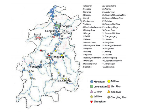
Water pollution prevention and control of the Xiang River has become an issue of great concern to China's central and local governments. To further analyze the effects of central and local governmental policies on water pollution prevention and control for the Xiang River, this study performs a big data analysis of 16 water quality parameters from 42 sections of the mainstream and major tributaries of the Xiang River, Hunan Province, China from 2005 to 2016. This study uses an evidential reasoning-based integrated assessment of water quality and principal component analysis, identifying the spatiotemporal changes in the primary pollutants of the Xiang River and exploring the correlations between potentially relevant factors. The analysis showed that a series of environmental protection policies implemented by Hunan Province since 2008 have had a significant and targeted impact on annual water quality pollutants in the mainstream and tributaries. In addition, regional industrial structures and management policies also have had a significant impact on regional water quality. The results showed that, when examining the changes in water quality and the effects of pollution control policies, a big data analysis of water quality monitoring results can accurately reveal the detailed relationships between management policies and water quality changes in the Xiang River. Compared with policy impact evaluation methods primarily based on econometric models, such a big data analysis has its own advantages and disadvantages, effectively complementing the traditional methods of policy impact evaluations. Policy impact evaluations based on big data analysis can further improve the level of refined management by governments and provide a more specific and targeted reference for improving water pollution management policies for the Xiang River.

References

[1]	S. Shao, X. Li, J. Cao, L. Yang, China's economic policy choices for governing smog pollution based on spatial spillover effects, Econ. Res. J., 51 (2016), 73–88.
[2]	D. Ghernaout, M. Aichouni, A. Alghamdi, Applying big data in water treatment industry: A new era of advance, Int. J. Adv. Appl. Sci., 5 (2018), 89–97. https://doi.org/10.21833/ijaas.2018.03.013 doi: 10.21833/ijaas.2018.03.013
[3]	J. Wu, S. Guo, J. Li, D. Zeng, Big data meet green challenges: Big data toward green applications, IEEE Syst. J., 10 (2016), 888–900. https://doi.org/10.1109/JSYST.2016.2550530 doi: 10.1109/JSYST.2016.2550530
[4]	Y. Liu, P. Failler, Z. Liu, Impact of environmental regulations on energy efficiency: A case study of China's air pollution prevention and control action plan, Sustainability, 14 (2022). https://doi.org/10.3390/su14063168 doi: 10.3390/su14063168
[5]	T. Wen, X. Niu, M. Gonzales, G. Zheng, Z. Li, S. L. Brantley, Big groundwater data sets reveal possible rare contamination amid otherwise improved water quality for some analytes in a region of Marcellus shale development, Environ. Sci. Technol., 52 (2018), 7149–7159. https://doi.org/10.1021/acs.est.8b01123 doi: 10.1021/acs.est.8b01123
[6]	H. Wang, Can voluntary environmental policy approaches be effective in Chinese context, China Popul., Resour. Environ., 20 (2010), 89–94.
[7]	Z. Li, F. Zou, B. Mo, Does mandatory CSR disclosure affect enterprise total factor productivity, Econ. Res.-Ekonomska Istraživanja, 35 (2021), 4902–4921. https://doi.org/10.1080/1331677x.2021.2019596 doi: 10.1080/1331677x.2021.2019596
[8]	H. Zhang, G. Liu, H. Hao, Review, assessment and recommendations on environmental policy in western China, China Popul., Resour. Environ., 23 (2013), 44–51.
[9]	M. H. Hansen, H. Li, R. Svarverud, Ecological civilization: Interpreting the Chinese past, projecting the global future, Global Environ. Change, 53 (2018), 195–203. https://doi.org/10.1016/j.gloenvcha.2018.09.014 doi: 10.1016/j.gloenvcha.2018.09.014
[10]	R. D. Mohr, Technical change, external economies, and the Porter hypothesis, J. Environ. Econ. Manage., 43 (2002), 158–168. https://doi.org/10.1006/jeem.2000.1166 doi: 10.1006/jeem.2000.1166
[11]	P. West, P. Senez, Environmental assessment of the NAFTA: The mexican environmental regulation position, report prepared for the Province of British Columbia, Ministry of Economic Development, Small Bus. Trade, 1992 (1992), 69–70.
[12]	J. Liu, J. Ren, Y. Zhang, X. Peng, Y. Zhang, Y. Yang, Efficient dependent task offloading for multiple applications in MEC-cloud system, IEEE Trans. Mob. Comput., 22 (2021), 2147–2162. https://doi.org/10.1109/TMC.2021.3119200 doi: 10.1109/TMC.2021.3119200
[13]	M. Greenstone, R. Hanna, Environmental regulations, air and water pollution, and infant mortality in India, Am. Econ. Rev., 104 (2014), 3038–3072. https://doi.org/10.1257/aer.104.10.3038 doi: 10.1257/aer.104.10.3038
[14]	B. Laplante, P. Rilstone, Environmental inspections and emissions of the pulp and paper industry in Quebec, J. Environ. Econ. Manage., 31 (1996), 19–36. https://doi.org/10.1006/jeem.1996.0029 doi: 10.1006/jeem.1996.0029
[15]	D. Zavras, Healthcare access as an important element for the EU's socioeconomic development: Greece's residents' opinions during the COVID-19 pandemic, Natl. Account. Rev., 4 (2022), 362–377. https://doi.org/10.3934/nar.2022020 doi: 10.3934/nar.2022020
[16]	H. Wang, Comparison and selection of environmental regulation policy in China: based on Bayesian model averaging approach, China Popul., Resour. Environ., 26 (2016), 132–138.
[17]	A. J. Hedley, C. M. Wong, T. Q. Thach, S. Ma, T. H. Lam, H. R. Anderson, Cardiorespiratory and all-cause mortality after restrictions on sulphur content of fuel in Hong Kong: an intervention study, Lancet, 360 (2002), 1646–1652. https://doi.org/10.1016/S0140-6736(02)11612-6 doi: 10.1016/S0140-6736(02)11612-6
[18]	Z. Li, J. Zhu, J. He, The effects of digital financial inclusion on innovation and entrepreneurship: A network perspective, Electron. Res. Arch., 30 (2022), 4697–4715. https://doi.org/10.3934/era.2022238 doi: 10.3934/era.2022238
[19]	S. Tanaka, Environmental regulations on air pollution in China and their impact on infant mortality, J. Health Econ., 42 (2015), 90–103. https://doi.org/10.1016/j.jhealeco.2015.02.004 doi: 10.1016/j.jhealeco.2015.02.004
[20]	Y. Chen, A. Ebenstein, M. Greenstone, H. Li, Evidence on the impact of sustained exposure to air pollution on life expectancy from China's Huai River policy, PNAS, 110 (2013), 12936–12941. https://doi.org/10.1073/pnas.1300018110 doi: 10.1073/pnas.1300018110
[21]	Y. Liu, C. Ma, Z. Huang, Can the digital economy improve green total factor productivity? An empirical study based on Chinese urban data, Math. Biosci. Eng., 20 (2023), 6866–6893. https://doi.org/10.3934/mbe.2023296 doi: 10.3934/mbe.2023296
[22]	H. Wang, R. Zhang, Effects of environmental regulation on CO₂ emissions: An empirical analysis of 282 cities in China, Sustainable Prod. Consumption, 29 (2022), 259–272. https://doi.org/10.1016/j.spc.2021.10.016 doi: 10.1016/j.spc.2021.10.016
[23]	L. Yang, K. L. Wang, Regional differences of environmental efficiency of China's energy utilization and environmental regulation cost based on provincial panel data and DEA method, Math. Comput. Model., 58 (2013), 1074–1083. https://doi.org/10.1016/j.mcm.2012.04.004 doi: 10.1016/j.mcm.2012.04.004
[24]	H. Tanaka, C. Tanaka, Sustainable investment strategies and a theoretical approach of multi-stakeholder communities, Green Finance, 4 (2022), 329–346. https://doi.org/10.3934/gf.2022016 doi: 10.3934/gf.2022016
[25]	T. Li, J. Wen, D. Zeng, K. Liu, Has enterprise digital transformation improved the efficiency of enterprise technological innovation? A case study on Chinese listed companies, Math. Biosci. Eng., 19 (2022), 12632–12654. https://doi.org/10.3934/mbe.2022590 doi: 10.3934/mbe.2022590
[26]	S. Ren, X. Li, B. Yuan, D. Li, X. Chen, The effects of three types of environmental regulation on eco-efficiency: A cross-region analysis in China, J. Clean Prod., 173 (2018), 245–255. https://doi.org/10.1016/j.jclepro.2016.08.113 doi: 10.1016/j.jclepro.2016.08.113
[27]	J. Liu, Y. Zhang, J. Ren, Y. Zhang, Auction-based dependent task offloading for IoT users in edge clouds, IEEE Internet Things, 2022 (2022). https://doi.org/10.1109/JIOT.2022.3221431 doi: 10.1109/JIOT.2022.3221431
[28]	Kanupriya, Indian textile sector, competitiveness, gender and the digital circular economy: A critical perspective, Natl. Account. Rev., 4 (2022), 237–250. https://doi.org/10.3934/nar.2022014 doi: 10.3934/nar.2022014
[29]	Z. Chu, C. Bian, C. Liu, J. Zhu, Evolutionary game analysis on haze governance in Beijing-Tianjin-Hebei: Based on a simulation tool for proposed environmental regulation policies, China Popul., Resour. Environ., 28 (2018), 63–75.
[30]	B. Ma, X. Lv, X. Chen, X. Chen, Analysis of atmospheric emission monitoring big data of thermal power plants and study on the policy impact, China Popul., Resour. Environ., 29 (2019), 73–79.
[31]	Y. Liu, L. Chen, L. Lv, P. Failler, The impact of population aging on economic growth: A case study on China, AIMS Math., 8 (2023), 10468–10485. https://doi.org/10.3934/math.2023531 doi: 10.3934/math.2023531
[32]	Y. Xu, Changes and developing trend of China's marine governance policy: An empirical research based on 161 policy texts from 1982 to 2015, China Popul., Resour. Environ., 28 (2018), 165–176.
[33]	Y. Wang, M. Li, Study on local government attention of ecological environment governance: Based on the text analysis of government work report in 30 provinces and cities (2006–2015), China Popul., Resour. Environ., 27 (2017), 28–35.
[34]	W. Guo, B. Xi, C. Huang, J. Li, Z. Tang, W. Li, et al., Solid waste management in China: Policy and driving factors in 2004–2019, Resour. Conserv. Recycl., 173 (2021), 105727. https://doi.org/10.1016/j.resconrec.2021.105727 doi: 10.1016/j.resconrec.2021.105727
[35]	T. Li, X. Li, G. Liao, Business cycles and energy intensity. Evidence from emerging economies, Borsa Istanbul Rev., 22 (2022), 560–570. https://doi.org/10.1016/j.bir.2021.07.005 doi: 10.1016/j.bir.2021.07.005
[36]	P. Zweifel, Expanding insurability through exploiting linear partial information, Data Sci. Finance Econ., 2 (2022), 1–16. https://doi.org/10.3934/dsfe.2022001 doi: 10.3934/dsfe.2022001
[37]	Y. Liu, Z. Li, M. Xu, The influential factors of financial cycle spillover: Evidence from China, Emerg. Markets Finance Trade, 56 (2019), 1336–1350. https://doi.org/10.1080/1540496x.2019.1658076 doi: 10.1080/1540496x.2019.1658076
[38]	H. Yin, Z. Xu, Discussion on China's single-factor water quality assessment method, Water Purif. Technol., 27 (2008), 1–3.
[39]	Y. Wang, J. Yang, D. Xu, Environmental impact assessment using the evidential reasoning approach, Eur. J. Oper. Res., 174 (2006), 1885–1913. https://doi.org/10.1016/j.ejor.2004.09.059 doi: 10.1016/j.ejor.2004.09.059
[40]	Y. Zhang, X. Deng, D. Wei, Y. Deng, Assessment of E-Commerce security using AHP and evidential reasoning, Expert Syst. Appl., 39 (2012), 3611–3623. https://doi.org/10.1016/j.eswa.2011.09.051 doi: 10.1016/j.eswa.2011.09.051
[41]	J. Gorin, Assessment as evidential reasoning, Teach. Coll. Rec., 116 (2014), 1–26. https://doi.org/10.1177/016146811411601101 doi: 10.1177/016146811411601101
[42]	Z. Li, Z. Huang, Y. Su, New media environment, environmental regulation and corporate green technology innovation: Evidence from China, Energy Econ., 119 (2023). https://doi.org/10.1016/j.eneco.2023.106545 doi: 10.1016/j.eneco.2023.106545
[43]	X. Si, C. Hu, J. Yang, Q. Zhang, On the dynamic evidential reasoning algorithm for fault prediction, Expert Syst. Appl., 38 (2011), 5061–5080. https://doi.org/10.1016/j.eswa.2010.09.144 doi: 10.1016/j.eswa.2010.09.144
[44]	Y. Liu, P. Failler, Y. Ding, Enterprise financialization and technological innovation: Mechanism and heterogeneity, PLoS One, 17 (2022), e0275461. https://doi.org/10.1371/journal.pone.0275461 doi: 10.1371/journal.pone.0275461
[45]	J. Lein, Applying evidential reasoning methods to agricultural land cover classification, Int. J. Remote Sens., 24 (2003), 4161–4180. https://doi.org/10.1080/0143116031000095916 doi: 10.1080/0143116031000095916
[46]	C. Yu, Z. Li, Z. Yang, A universal calibrated model for the evaluation of surface water and groundwater quality: Model development and a case study in China, J. Environ. Manage., 163 (2015), 20–27. https://doi.org/10.1016/j.jenvman.2015.07.011 doi: 10.1016/j.jenvman.2015.07.011
[47]	G. Li, X. Liu, Z. Liu, W. Guo, Water quality assessment of main rivers in Tianjin based on principal component analysis and water quality identification index, J. Ecol. Rural Environ., 27 (2011), 27–31.
[48]	J. B. Yang, D. L. Xu, Evidential reasoning rule for evidence combination, Artif. Intell., 205 (2013), 1–29. https://doi.org/10.1016/j.artint.2013.09.003 doi: 10.1016/j.artint.2013.09.003
[49]	J. B. Yang, M. G. Singh, An evidential reasoning approach for multiple-attribute decision making with uncertainty, IEEE Trans. Syst. Man Cybern., 24 (1994), 1–18. https://doi.org/10.1109/21.259681 doi: 10.1109/21.259681
[50]	H. Chu, W. Lu, L. Zhang, Application of artificial neural network in environmental water quality assessment, J. Agric. Sci. Technol., 15 (2013), 343–356.
[51]	Y. Liu, J. Liu, L. Zhang, Enterprise financialization and R & D innovation: A case study of listed companies in China, Electron. Res. Arch., 31 (2023), 2447–2471. https://doi.org/10.3934/era.2023124 doi: 10.3934/era.2023124
[52]	G. Shafer, A Mathematical Theory of Evidence, Princeton University Press, 1976.

Reader Comments

Your name:*

Email:*
© 2023 the Author(s), licensee AIMS Press. This is an open access article distributed under the terms of the Creative Commons Attribution License (http://creativecommons.org/licenses/by/4.0)