Runoff forecasting model based on variational mode decomposition and artificial neural networks

Xin Jing; Jungang Luo; Shangyao Zhang; Na Wei; Xin Jing; Jungang Luo; Shangyao Zhang; Na Wei

doi:10.3934/mbe.2022076

Mathematical Biosciences and Engineering

2022, Volume 19, Issue 2: 1633-1648. doi: 10.3934/mbe.2022076

Previous Article Next Article

Research article Special Issues

Runoff forecasting model based on variational mode decomposition and artificial neural networks

State Key Laboratory of Eco-hydraulics in Northwest Arid Region, Xi'an University of Technology, Shaanxi 710048, China

Academic Editor: Runzhang Xu

Received: 30 September 2021 Accepted: 29 November 2021 Published: 13 December 2021

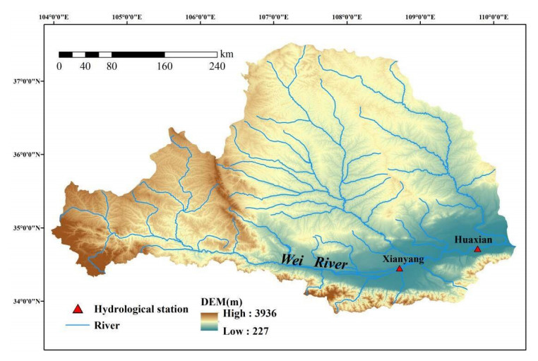
Accurate runoff forecasting plays a vital role in water resource management. Therefore, various forecasting models have been proposed in the literature. Among them, the decomposition-based models have proved their superiority in runoff series forecasting. However, most of the models simulate each decomposition sub-signals separately without considering the potential correlation information. A neoteric hybrid runoff forecasting model based on variational mode decomposition (VMD), convolution neural networks (CNN), and long short-term memory (LSTM) called VMD-CNN-LSTM, is proposed to improve the runoff forecasting performance further. The two-dimensional matrix containing both the time delay and correlation information among sub-signals decomposing by VMD is firstly applied to the CNN. The feature of the input matrix is then extracted by CNN and delivered to LSTM with more potential information. The experiment performed on monthly runoff data investigated from Huaxian and Xianyang hydrological stations at Wei River, China, demonstrates the VMD-superiority of CNN-LSTM to the baseline models, and robustness and stability of the forecasting of the VMD-CNN-LSTM for different leading times.

Keywords:

Citation: Xin Jing, Jungang Luo, Shangyao Zhang, Na Wei. Runoff forecasting model based on variational mode decomposition and artificial neural networks[J]. Mathematical Biosciences and Engineering, 2022, 19(2): 1633-1648. doi: 10.3934/mbe.2022076

Related Papers:

[1]	Nitesha Dwarika . The risk-return relationship in South Africa: tail optimization of the GARCH-M approach. Data Science in Finance and Economics, 2022, 2(4): 391-415. doi: 10.3934/DSFE.2022020
[2]	Moses Khumalo, Hopolang Mashele, Modisane Seitshiro . Quantification of the stock market value at risk by using FIAPARCH, HYGARCH and FIGARCH models. Data Science in Finance and Economics, 2023, 3(4): 380-400. doi: 10.3934/DSFE.2023022
[3]	Xiaoling Chen, Xingfa Zhang, Yuan Li, Qiang Xiong . Daily LGARCH model estimation using high frequency data. Data Science in Finance and Economics, 2021, 1(2): 165-179. doi: 10.3934/DSFE.2021009
[4]	Samuel Asante Gyamerah, Collins Abaitey . Modelling and forecasting the volatility of bitcoin futures: the role of distributional assumption in GARCH models. Data Science in Finance and Economics, 2022, 2(3): 321-334. doi: 10.3934/DSFE.2022016
[5]	Changlin Wang . Different GARCH model analysis on returns and volatility in Bitcoin. Data Science in Finance and Economics, 2021, 1(1): 37-59. doi: 10.3934/DSFE.2021003
[6]	Alexandra Piryatinska, Boris Darkhovsky . Retrospective technology of segmentation and classification for GARCH models based on the concept of the $\epsilon$ -complexity of continuous functions. Data Science in Finance and Economics, 2022, 2(3): 237-253. doi: 10.3934/DSFE.2022012
[7]	Kasra Pourkermani . VaR calculation by binary response models. Data Science in Finance and Economics, 2024, 4(3): 350-361. doi: 10.3934/DSFE.2024015
[8]	Changlin Wang . Correction: Different GARCH models analysis of returns and volatility in Bitcoin. Data Science in Finance and Economics, 2022, 2(3): 205-208. doi: 10.3934/DSFE.2022010
[9]	Deniz Sevinç . Volatility spillovers among MIST stock markets. Data Science in Finance and Economics, 2022, 2(2): 80-95. doi: 10.3934/DSFE.2022004
[10]	Katleho Makatjane, Ntebogang Moroke . Examining stylized facts and trends of FTSE/JSE TOP40: a parametric and Non-Parametric approach. Data Science in Finance and Economics, 2022, 2(3): 294-320. doi: 10.3934/DSFE.2022015

Abstract

1. Introduction

Asymmetric datasets modeling utilizing generalized continuous distributions is quite an interesting area of research in recent times, and quite a number of generalized continuous distributions have been proposed, established and utilized in different fields of study. Besides with the new progressions in probability distribution theory, more vigorous forms of continuous distributions have been proposed utilizing the exponentiated method, transformer-transformer method, beta-generated method and gamma-generated method, among others. Shockingly, these recent distributions have been valuable in resolving issues in different fields of study other than in GARCH-type volatility models. Along these lines, it is important to develop new conditional innovation distributions capable of handling both significant skewness and excess kurtosis present in financial asset returns. Jones (2001) proposed a simplified extension of the symmetric Student's-t distribution known as the skew-t distribution to handle real-life asymmetric datasets. Jones and Faddy (2003) described the distribution as a simplified skew-t distribution and provided some important structural properties. Some other forms of the skew-t distribution that have been developed can be found in the literature (Johnson et al., 1995; Sahu et al., 2003; Azzalini and Capitanio, 2003). More so, the statistical literature consists several extended forms of the skew-t distribution. For example, the generalized hyperbolic skew-t distribution (Aas and Haff, 2006), beta skew-t distribution (Shittu et al., 2014), Balakrishnan skew-t distribution (Shafiei and Doostparast, 2014), Kumaraswamy skew-t distribution (Khamis et al., 2017), exponentiated skew-t distribution (Dikko and Agboola, 2017), generalized alpha skew-t distribution (Altun et al., 2018), odd exponentiated skew-t distribution (Adubisi et al., 2021a), and type I half-logistic skew-t distribution (Adubisi et al., 2021b).

For any baseline distribution with parameter vector $\zeta$ , proposed the exponentiated half-logistic-G (EHL-G) family based on the T-X method (). Given that $k\left(t\right)$ and $K\left(t\right)$ are the probability density function (pdf) and cumulative distribution function (cdf) of a random variable (r.v) $T\in \left[c, d\right]$ for $\left[c, d\right]\in \left(-\infty, +\infty \right)$ , respectively. Let $R\left[H\left(y;\zeta \right)\right]$ be a function of the cdf of another r. v Y satisfying the following conditions: [i] $R\left[H\left(y;\zeta \right)\right]\in \left[c, d\right]$ ; [ii] $R\left[H\left(y;\zeta \right)\right]\to c$ as $y\to -\infty$ and $R\left[H\left(y;\zeta \right)\right]\to d$ as $y\to \infty$ ; and [iii] $R\left[H\left(y;\zeta \right)\right]$ is differentiable and monotonically non-decreasing. The cdf of the T-X method is given by

$F\left(y\right) = {\int }_{c}^{R\left[H\left(y;\zeta \right)\right]}\begin{array}{cc}& k\left(t\right)dt = K\left(R\left[H\left(y;\zeta \right)\right]\right)\end{array},$

(1)

Setting $\begin{array}{cc}k\left(t\right) = \frac{2\alpha \varphi {e}^{-\alpha t}{\left[1-{e}^{-\alpha t}\right]}^{\varphi -1}}{{\left(1+{e}^{-\alpha t}\right)}^{\varphi +1}}, & t > 0, \end{array}$ where $\alpha, \varphi > 0$ are the shape parameters, and

$21R\left[H\left(y;\zeta \right)\right] = - \ \mathit{log} \ \left[1-H\left(y;\zeta \right)\right]$ , the cdf of the EHL-G family is given by

$F(y;\alpha, \varphi, \zeta) = {\left\{\frac{1-{\left[1-H\left(y;\zeta \right)\right]}^{\alpha }}{1+{\left[1-H\left(y;\zeta \right)\right]}^{\alpha }}\right\}}^{\varphi },$

(2)

and the corresponding pdf to Equation 2 is

$f(y;\alpha, \varphi, \zeta) = 2\alpha \varphi h\left(y;\zeta \right){\left[1-H\left(y;\zeta \right)\right]}^{\alpha -1}\frac{{\left\{1-{\left[1-H\left(y;\zeta \right)\right]}^{\alpha }\right\}}^{\varphi -1}}{{\left\{1+{\left[1-H\left(y;\zeta \right)\right]}^{\alpha }\right\}}^{\varphi +1}},$

(3)

where $\alpha, \varphi > 0$ are two additional shape parameters. $H\left(y;\zeta \right)$ and $h\left(y;\zeta \right)$ are the baseline cdf and pdf.

In this research work, a hybrid form of the skew-t distribution developed by using the exponentiated half logistic-G family of distributions is proposed. The new three-parameter model called the exponentiated half logistic skew t (EHL_ST) distribution appropriate for modeling right or left skewed and heavy-tailed datasets is developed. By inserting the skew-t cdf $H\left(y;\kappa \right) = \frac{1}{2}\left(1+\frac{y}{\sqrt{\kappa +{y}^{2}}}\right)$ into Equation 2 leads to

$F\left(y\right) = {\left\{\frac{1-{\left[1-\left(\frac{1}{2}\left(1+\frac{y}{\sqrt{\kappa +{y}^{2}}}\right)\right)\right]}^{\alpha }}{1+{\left[1-\left(\frac{1}{2}\left(1+\frac{y}{\sqrt{\kappa +{y}^{2}}}\right)\right)\right]}^{\alpha }}\right\}}^{\varphi },$

(4)

The corresponding pdf to Equation 4 is

$f\left(y\right) = \frac{2\alpha \varphi \kappa {\left[1-\left(\frac{1}{2}\left(1+\frac{y}{\sqrt{\kappa +{y}^{2}}}\right)\right)\right]}^{\alpha -1}{\left\{1-{\left[1-\left(\frac{1}{2}\left(1+\frac{y}{\sqrt{\kappa +{y}^{2}}}\right)\right)\right]}^{\alpha }\right\}}^{\varphi -1}}{2{\left(\kappa +{y}^{2}\right)}^{\frac{3}{2}}{\left\{1+{\left[1-\left(\frac{1}{2}\left(1+\frac{y}{\sqrt{\kappa +{y}^{2}}}\right)\right)\right]}^{\alpha }\right\}}^{\varphi +1}},$

(5)

where $\alpha > 0$ and $\varphi > 0$ are two shape parameters, and $\kappa$ denote the skew parameter. From now onward, $Y\sim EH{L}_{ST}\left(\alpha, \varphi, \kappa \right)$ denotes a random variable with pdf Equation 5. The hazard rate function (hrf) of Y is

$\eta \left(y\right) = \frac{\alpha \varphi \left(\frac{\kappa }{{\left(\kappa +{y}^{2}\right)}^{\frac{3}{2}}}\right){\left[1-\left(\frac{1}{2}\left(1+\frac{y}{\sqrt{\kappa +{y}^{2}}}\right)\right)\right]}^{\alpha -1}{\left\{1-{\left[1-\left(\frac{1}{2}\left(1+\frac{y}{\sqrt{\kappa +{y}^{2}}}\right)\right)\right]}^{\alpha }\right\}}^{\varphi -1}}{\left({\left\{1+{\left[1-\left(\frac{1}{2}\left(1+\frac{y}{\sqrt{\kappa +{y}^{2}}}\right)\right)\right]}^{\alpha }\right\}}^{\varphi }-{\left\{1-{\left[1-\left(\frac{1}{2}\left(1+\frac{y}{\sqrt{\kappa +{y}^{2}}}\right)\right)\right]}^{\alpha }\right\}}^{\varphi }\left\{1+{\left[1-\left(\frac{1}{2}\left(1+\frac{y}{\sqrt{\kappa +{y}^{2}}}\right)\right)\right]}^{\alpha }\right\}\right)} .$

(6)

Detailed properties of the EHL_ST model can be found in Adubisi et al. (2021c). Lately, there has been a key interest in the comparison of different estimation procedures for the parameter estimation of several distributions. For example, the extended exponential geometric (Louzada et al., 2016), Binomial exponential 2 (Bakouch et al., 2017), Poisson exponential (Rodrigues et al., 2018), type-I half-logistic Top-Leone (ZeinEldin et al., 2019), polynomial exponential (Chesneau et al., 2020), Fréchet (Ramos et al., 2020), odd exponential half-logistic exponential (Aldahlan and Afify, 2020), among others. The motivation in developing the new model is to create a more flexible heavy-tailed distribution with right-skewed, left-skewed, symmetric and unimodal features capable of handling the stylized features in financial datasets. The aim of this work is to estimate the parameters of the EHL_ST distribution using different frequentist estimation criterions such as the maximum likelihood, Anderson-Darling, maximum product of spacing, ordinary least squares, Cramer-von mises and weighted least squares. These estimation criterions using extensive Monte Carlo simulation are compared to discourse their performance. Also, Altun (2019) noted that the assumption of the conditional innovation density of the GARCH volatility model directly impacts on the accuracy of volatility predictions. Hence, the standardized form of the EHL_ST model is also derived to serve as an alternative conditional innovation density in modeling and forecasting the volatility of the inflation rates in sub-Sahara Africa, specifically Nigeria inflation rate using the GARCH-type volatility models. The rest of this research work is designed as follows. The quantile function of the EHL_ST is derived in Section 2. Six estimation criterions for estimating the parameters of the EHL_ST model are presented in Section 3. Simulation study to compare these criterions and real-life application are presented in Section 4. The application of the EHL_ST density in volatility modeling is illustrated via GARCH-type models in Section 5. The empirical results of the GARCH process are presented in Section 6. Conclusion of the work in Section 7.

Figures 1 and 2 provides plots of the pdf and hazard rate function of the EHL_ST distribution for selected values of the parameters. The plot in figure 2, shows that the hazard rate function can be J-shape, increasing and decreasing.

Figure 1. The EHL_ST density (pdf) plots for selected parameter values.

DownLoad: Full-Size Img PowerPoint

Figure 2. The EHL_ST hazard rate function (hrf) plots for selected parameter values.

DownLoad: Full-Size Img PowerPoint

2. Quantile function

The quantile function, $Q\left(u\right) = {F}^{-1}\left(u\right)$ of Y can be derived by inverting Equation 4. The quantile function of the EHL_ST distribution takes the form:

$\begin{array}{ccc}Q\left(u\right) = {\kappa }^{\frac{1}{2}}\frac{\left[1-2{\left(\frac{1-{u}^{\frac{1}{\varphi }}}{1+{u}^{\frac{1}{\varphi }}}\right)}^{\frac{1}{\alpha }}\right]}{{\left[1-{\left(1-2{\left(\frac{1-{u}^{\frac{1}{\varphi }}}{1+{u}^{\frac{1}{\varphi }}}\right)}^{\frac{1}{\alpha }}\right)}^{2}\right]}^{\frac{1}{2}}}, & & 0\le u\le 1.\end{array}$

(7)

The quantile function in Equation 7 can define various quantile measures such as Bowley's skewness and Moor's kurtosis of the EHL_ST distribution. depicts the three-dimensional plots of these skewness and kurtosis measures. It is clear that the skewness was increasing in $\varphi$ and decreasing in $\alpha$ while the kurtosis is increasing in $\alpha$ and decreasing in $\varphi$ , and were independent of $\kappa$ .

Figure 3. Bowley's skewness and Moor's kurtosis plots of the EHL_ST distribution.

DownLoad: Full-Size Img PowerPoint

3. Methods of estimation

This section discusses six estimation criterions, these are the maximum likelihood (ML), maximum product of spacing (MPS), Anderson-Darling (ANDA), ordinary least squares (OLS), weighted least squares (WLS) and Cramer-von Mises (CVM) to estimate the new model parameters.

3.1. Maximum likelihood

The ML estimation is considered the best for estimating distribution parameters given its excellent characteristics. Let ${y}_{1}, \dots, {y}_{T}$ be the observed values of sizes (T) from the EHL_ST distribution. The log-likelihood function derived from Equation 6 is given by

$l\left(\alpha, \varphi, \kappa \right) = T \ \mathit{ln} \ \alpha +T \ \mathit{ln} \ \varphi +T \ \mathit{ln} \ \kappa \\ -\frac{3}{2}\sum\limits _{k = 1}^{T} \ \mathit{ln} \ \left(\kappa +{y}_{k}^{2}\right)+\left(\alpha -1\right)\sum\limits _{k = 1}^{T} \ \mathit{ln} \ \left({z}_{k}\right)+\left(\varphi -1\right)\sum\limits _{k = 1}^{T} \ \mathit{ln} \ \left(1-{\left({z}_{k}\right)}^{\alpha }\right) \\ \begin{array}{ccccccccccccccc} -\left(\varphi +1\right)\sum\nolimits _{k = 1}^{T} \ \mathit{ln} \ \left(1+{\left({z}_{k}\right)}^{\alpha }\right)\end{array}$

(8)

$\text{where } {z}_{k} = \left(1-\frac{1}{2}\left(1+\frac{{y}_{k}}{\sqrt{\kappa +{y}_{k}^{2}}}\right)\right)$

(9)

Let ${\widehat{\alpha }}_{MLE}, {\widehat{\varphi }}_{MLE}$ and ${\widehat{\kappa }}_{MLE}$ be the ML estimates of $\alpha, \varphi$ and $\kappa$ . These can be obtained numerically by maximizing $l\left(\alpha, \varphi, \kappa \right)$ or solving the following differential equations:

${U}_{\alpha } = \frac{T}{\alpha }+\sum\nolimits _{k = 1}^{T} \ \mathit{ln} \ \left({z}_{k}\right)-\left(\varphi -1\right)\sum\nolimits _{k = 1}^{T}\frac{{\left({z}_{k}\right)}^{\alpha } \ \mathit{ln} \ \left({z}_{k}\right)}{\left\{1-{\left({z}_{k}\right)}^{\alpha }\right\}}-\left(\varphi +1\right)\sum\nolimits _{k = 1}^{T}\frac{{\left({z}_{k}\right)}^{\alpha } \ \mathit{ln} \ \left({z}_{k}\right)}{\left\{1+{\left({z}_{k}\right)}^{\alpha }\right\}} = 0,$

(10)

${U}_{\varphi } = \frac{T}{\varphi }+\sum\nolimits _{k = 1}^{T} \ \mathit{ln} \ \left(1-{\left({z}_{k}\right)}^{\alpha }\right)-\sum\nolimits _{k = 1}^{T} \ \mathit{ln} \ \left\{1+{\left({z}_{k}\right)}^{\alpha }\right\} = 0,$

(11)

and

${U}_{\eta } = \frac{T}{\kappa }-\frac{3}{2}\sum\limits _{k = 1}^{T}\frac{1}{\left(\kappa +{y}_{k}^{2}\right)}+\left(\alpha -1\right)\sum\limits _{k = 1}^{T}\frac{{y}_{k}}{4{\left(\kappa +{y}_{k}^{2}\right)}^{\frac{3}{2}}\left({z}_{k}\right)}\\ -\alpha \left(\varphi -1\right)\sum\limits _{k = 1}^{T}\frac{{y}_{k}{\left({z}_{k}\right)}^{\alpha }}{4{\left(\kappa +{y}_{k}^{2}\right)}^{\frac{3}{2}}\left({z}_{k}\right)\left\{1+{\left({z}_{k}\right)}^{\alpha }\right\}} \\ \begin{array}{cccc} -\alpha \left(\varphi +1\right)\sum\nolimits _{k = 1}^{T}\frac{{y}_{k}{\left({z}_{k}\right)}^{\alpha }}{4{\left(\kappa +{y}_{k}^{2}\right)}^{\frac{3}{2}}\left({z}_{k}\right)\left\{1+{\left({z}_{k}\right)}^{\alpha }\right\}}\end{array} = 0$

(12)

3.2. Ordinary least squares

Let ${y}_{\left(1:T\right)}, {y}_{\left(2:T\right)}, \dots, {y}_{\left(T:T\right)}$ be the ordered sample of size (T) from the EHL_ST distribution with cdf in Equation 5. The OLS estimates ${\widehat{\alpha }}_{OLS}, {\widehat{\varphi }}_{OLS}$ and ${\widehat{\kappa }}_{OLS}$ of $\alpha, \varphi$ and $\kappa$ can be obtained numerically by minimizing

$OL\left(\alpha, \varphi, \kappa \right) = \sum\nolimits _{k = 1}^{T}{\left[{\left\{\frac{1-{\left[1-\left(\frac{1}{2}\left(1+\frac{{y}_{\left(k:T\right)}}{\sqrt{\kappa +{y}_{\left(k:T\right)}^{2}}}\right)\right)\right]}^{\alpha }}{1+{\left[1-\left(\frac{1}{2}\left(1+\frac{{y}_{\left(k:T\right)}}{\sqrt{\kappa +{y}_{\left(k:T\right)}^{2}}}\right)\right)\right]}^{\alpha }}\right\}}^{\varphi }-\wp (k, T)\right]}^{2},$

(13)

where $\wp (k, T) = \frac{\left(T+1-k\right)}{\left(T+1\right)}$ , with respect to $\alpha, \varphi$ and $\kappa$ .Also, the model estimates can be obtained by solving the following differential equations:

$\frac{\partial OL\left(\alpha, \varphi, \kappa \right)}{\partial \alpha } = \sum\nolimits _{k = 1}^{T}\left[{\left\{\frac{1-{\left[{z}_{(k:T)}\right]}^{\alpha }}{1+{\left[{z}_{(k:T)}\right]}^{\alpha }}\right\}}^{\varphi }-\wp (k, T)\right]{\varPhi }_{1}\left({y}_{(k:T)}\left|\alpha, \varphi, \kappa \right.\right) = 0,$

(14)

$\frac{\partial OL\left(\alpha, \varphi, \kappa \right)}{\partial \varphi } = \sum\nolimits _{k = 1}^{T}\left[{\left\{\frac{1-{\left[{z}_{(k:T)}\right]}^{\alpha }}{1+{\left[{z}_{(k:T)}\right]}^{\alpha }}\right\}}^{\varphi }-\wp (k, T)\right]{\varPhi }_{2}\left({y}_{(k:T)}\left|\alpha, \varphi, \kappa \right.\right) = 0,$

(15)

and

$\frac{\partial OL\left(\alpha, \varphi, \kappa \right)}{\partial \kappa } = \sum\nolimits _{k = 1}^{T}\left[{\left\{\frac{1-{\left[{z}_{(k:T)}\right]}^{\alpha }}{1+{\left[{z}_{(k:T)}\right]}^{\alpha }}\right\}}^{\varphi }-\wp (k, T)\right]{\varPhi }_{3}\left({y}_{(k:T)}\left|\alpha, \varphi, \kappa \right.\right) = 0,$

(16)

where ${z}_{(k:T)}$ is the order transformed value of ${z}_{k}$ given by Equation 9, and

${\varPhi }_{1}\left({y}_{\left(k:T \ \ \right) \ \ }\left|\alpha, \varphi, \kappa \right.\right) = \frac{\left\{{\left(\frac{1-({z}_{(k:T \ ) \ \ \ }{)}^{\alpha }}{1+({z}_{(k:T \ ) \ \ \ }{)}^{\alpha }}\right)}^{\varphi }\varphi \left(\begin{array}{c}-\frac{\left({z}_{(k:T \ ) \ \ \ }{)}^{\alpha } \ \mathit{log} \ ({z}_{(k:T \ ) \ \ \ }\right)}{1+({z}_{(k:T \ ) \ \ \ }{)}^{\alpha }}\\ -\frac{\left[1-({z}_{(k:T \ ) \ \ \ }{)}^{\alpha } \ \ \right]\left({z}_{(k:T \ ) \ \ \ }{)}^{\alpha } \ \mathit{log} \ ({z}_{(k:T \ ) \ \ \ }\right)}{{\left[1+({z}_{(k:T \ ) \ \ \ }{)}^{\alpha } \ \ \right]}^{ \ \ 2}}\end{array}\right)\left[1+({z}_{(k:T \ ) \ \ \ }{)}^{\alpha } \ \ \right]\right\}}{1-({z}_{(k:T \ ) \ \ \ }{)}^{\alpha }}$

(17)

${\varPhi }_{2}\left({y}_{\left(k:T \ \ \right) \ \ }\left|\alpha, \varphi, \kappa \right.\right) = {\left(\frac{1-({z}_{(k:T \ ) \ \ \ }{)}^{\alpha }}{1+({z}_{(k:T \ ) \ \ \ }{)}^{\alpha }}\right)}^{\varphi } \ \mathit{log} \ \left(\frac{1-({z}_{(k:T \ ) \ \ \ }{)}^{\alpha }}{1+({z}_{(k:T \ ) \ \ \ }{)}^{\alpha }}\right)$

(18)

and

${\varPhi }_{3}\left({y}_{\left(k:T \ \ \right) \ \ }\left|\alpha, \varphi, \kappa \right.\right) = \frac{\left\{{\left(\frac{1-({z}_{(k:T \ ) \ \ \ }{)}^{\alpha }}{1+({z}_{(k:T \ ) \ \ \ }{)}^{\alpha }}\right)}^{\varphi }\varphi \left(\begin{array}{c}-\frac{\alpha y({z}_{(k:T \ ) \ \ \ }{)}^{\alpha }}{4{\left(\kappa +{y}_{(k:T \ ) \ \ \ }^{2}\right)}^{\frac{3}{2}}\left({z}_{(k:T \ ) \ \ \ }\right)\left[1+({z}_{(k:T \ ) \ \ \ }{)}^{\alpha } \ \ \right]}\\ -\frac{\alpha y\left[1-({z}_{(k:T \ ) \ \ \ }{)}^{\alpha } \ \ \right]({z}_{(k:T \ ) \ \ \ }{)}^{\alpha }}{4{\left[1+({z}_{(k:T \ ) \ \ \ }{)}^{\alpha } \ \ \right]}^{2}{\left(\kappa +{y}_{(k:T \ ) \ \ \ }^{2}\right)}^{\frac{3}{2}}\left({z}_{(k:T \ ) \ \ \ }\right)}\end{array}\right)\left[1+({z}_{(k:T \ ) \ \ \ }{)}^{\alpha } \ \ \right]\right\}}{1-({z}_{(k:T \ ) \ \ \ }{)}^{\alpha }}$

(19)

3.3. Weighted least squares

Applying the same symbolization as in the preceding subsection, the WLS estimates ${\widehat{\alpha }}_{WLS}, {\widehat{\varphi }}_{WLS}$ and ${\widehat{\kappa }}_{WLS}$ of $\alpha, \varphi$ and $\kappa$ can be obtained numerically by minimizing

$WL\left(\alpha, \varphi, \kappa \right) = \sum\nolimits _{k = 1}^{T}\varPsi (k, T){\left[{\left\{\frac{1-{\left[1-\left(\frac{1}{2}\left(1+\frac{{y}_{\left(k:T \ \ \right) \ \ }}{\sqrt{\kappa +{y}_{\left(k:T \ \ \right) \ \ }^{2}}}\right)\right) \ \ \right]}^{\alpha }}{1+{\left[1-\left(\frac{1}{2}\left(1+\frac{{y}_{\left(k:T \ \ \right) \ \ }}{\sqrt{\kappa +{y}_{\left(k:T \ \ \right) \ \ }^{2}}}\right)\right) \ \ \right]}^{\alpha }}\right\}}^{\varphi }-\wp (k, T) \ \ \right]}^{2},$

(20)

where $\varPsi (k, T) = \frac{{\left(T+1\right)}^{2}\left(T+2\right)}{k\left(T-k+1\right)}$ , relative to $\alpha, \varphi$ and $\kappa$ . Also, the model estimates can be obtained by solving the following differential equations:

$\frac{\partial WL\left(\alpha, \varphi, \kappa \right)}{\partial \alpha } = \sum\nolimits _{k = 1}^{T}\varPsi (k, T)\left[{\left\{\frac{1-{\left[{z}_{(k:T)}\right]}^{\alpha }}{1+{\left[{z}_{(k:T)}\right]}^{\alpha }}\right\}}^{\varphi }-\wp (k, T)\right]{\varPhi }_{1}\left({y}_{(k:T)}\left|\alpha, \varphi, \kappa \right.\right) = 0,$

(21)

$\frac{\partial WL\left(\alpha, \varphi, \kappa \right)}{\partial \varphi } = \sum\nolimits _{k = 1}^{T}\varPsi (k, T)\left[{\left\{\frac{1-{\left[{z}_{(k:T)}\right]}^{\alpha }}{1+{\left[{z}_{(k:T)}\right]}^{\alpha }}\right\}}^{\varphi }-\wp (k, T)\right]{\varPhi }_{2}\left({y}_{(k:T)}\left|\alpha, \varphi, \kappa \right.\right) = 0,$

(22)

and

$\frac{\partial OL\left(\alpha, \varphi, \kappa \right)}{\partial \kappa } = \sum\nolimits _{k = 1}^{T}\varPsi (k, T)\left[{\left\{\frac{1-{\left[{z}_{(k:T)}\right]}^{\alpha }}{1+{\left[{z}_{(k:T)}\right]}^{\alpha }}\right\}}^{\varphi }-\wp (k, T)\right]{\varPhi }_{3}\left({y}_{(k:T)}\left|\alpha, \varphi, \kappa \right.\right) = 0,$

(23)

where ${z}_{(k:T)}$ and ${\varPhi }_{i}\left({y}_{(k:T)}\left|\alpha, \varphi, \kappa \right.\right),$ $i = \mathrm{1, 2}, 3$ are given by Eqs 9, 17, 18 and 19, respectively.

3.4. Maximum product of spacing

, ) proposed the MPS estimator for the estimation of unknown parameters with ordered sample ${y}_{\left(1:T\right)}, {y}_{\left(2:T\right)}, \dots, {y}_{\left(T:T\right)}$ from the EHL_ST distribution and uniform spacing for this random sample is given by:

${D}_{k}\left(\alpha, \varphi, \kappa \right) = F\left({y}_{\left(k:T\right)}\left|\alpha, \varphi, \kappa \right.\right)-F\left({y}_{\left(k-1:T\right)}\left|\alpha, \varphi, \kappa \right.\right) \text{, for } k = \mathrm{1, 2}, \dots, T ,$

(24)

where $F\left({y}_{\left(0:T\right)}\left|\alpha, \varphi, \kappa \right.\right) = 0$ and $F\left({y}_{\left(T+1:T\right)}\left|\alpha, \varphi, \kappa \right.\right) = 1$ . The MPS estimates ${\widehat{\alpha }}_{MPS}$ , ${\widehat{\varphi }}_{MPS}$ and ${\widehat{\kappa }}_{MPS}$ of $\alpha, \varphi$ , and $\kappa$ can be obtained by maximizing

$MP\left(\alpha, \varphi, \kappa \right) = \frac{1}{T+1}\sum\nolimits _{k = 1}^{T+1} \ \mathit{log} \ ⟨{D}_{k}\left(\alpha, \varphi, \kappa \right)⟩$

(25)

relative to $\alpha, \varphi$ , and $\kappa$ . Also, the estimates can be obtained by solving the following differential equations:

$\frac{\partial MP\left(\alpha, \varphi, \kappa \right)}{\partial \alpha } = \sum\nolimits _{k = 1}^{T+1}\frac{1}{{D}_{k}\left(\alpha, \varphi, \kappa \right)}⟨{\varPhi }_{1}\left({y}_{\left(k:T\right)}\left|\alpha, \varphi, \kappa \right.\right)-{\varPhi }_{1}\left({y}_{\left(k-1:T\right)}\left|\alpha, \varphi, \kappa \right.\right)⟩ = 0,$

(26)

$\frac{\partial MP\left(\alpha, \varphi, \kappa \right)}{\partial \varphi } = \sum\nolimits _{k = 1}^{T+1}\frac{1}{{D}_{k}\left(\alpha, \varphi, \kappa \right)}⟨{\varPhi }_{2}\left({y}_{\left(k:T\right)}\left|\alpha, \varphi, \kappa \right.\right)-{\varPhi }_{2}\left({y}_{\left(k-1:T\right)}\left|\alpha, \varphi, \kappa \right.\right)⟩ = 0,$

(27)

and

$\frac{\partial MP\left(\alpha, \varphi, \kappa \right)}{\partial \kappa } = \sum\nolimits _{k = 1}^{T+1}\frac{1}{{D}_{k}\left(\alpha, \varphi, \kappa \right)}⟨{\varPhi }_{3}\left({y}_{\left(k:T\right)}\left|\alpha, \varphi, \kappa \right.\right)-{\varPhi }_{3}\left({y}_{\left(k-1:T\right)}\left|\alpha, \varphi, \kappa \right.\right)⟩ = 0$

(28)

where ${\varPhi }_{i}(.\left|\alpha, \varphi, \kappa \right.),$ $i = \mathrm{1, 2}, 3$ are specified in Equation s 17, 18 and 19, respectively.

3.5. Anderson-Darling

The ANDA estimates ${\widehat{\alpha }}_{ANDA}$ , ${\widehat{\varphi }}_{ANDA}$ and ${\widehat{\kappa }}_{ANDA}$ of the EHL_ST parameters can be obtained by minimizing relative to $\alpha, \varphi$ , and $\kappa$ , the function

${\rm A}D\left(\alpha, \varphi, \kappa \right) = -T-\frac{1}{T}\sum\nolimits _{k = 1}^{T}\left(2k-1\right)⟨ \ \mathit{log} \ \left[F\left({y}_{\left(k:T\right)}\left|\alpha, \varphi, \kappa \right.\right)\right]+ \ \mathit{log} \ \left[\stackrel{̄}{F}\left({y}_{\left(T+1-k:n\right)}\left|\alpha, \varphi, \kappa \right.\right)\right]⟩,$

(29)

Also, estimates obtained by solving the following nonlinear equations:

$\frac{\partial AD\left(\alpha, \varphi, \kappa \right)}{\partial \alpha } = \sum\nolimits _{k = 1}^{T}\left(2k-1\right)\left[\frac{{\varPhi }_{1}\left({y}_{\left(k:T \ \ \right) \ \ \ \ }\left|\alpha, \varphi, \kappa \right.\right)}{F\left({y}_{\left(k:T \ \ \right) \ \ \ \ }\left|\alpha, \varphi, \kappa \right.\right)}-\frac{{\varPhi }_{1}\left({y}_{\left(T+1-k:T \ \ \right) \ \ \ \ }\left|\alpha, \varphi, \kappa \right.\right)}{\stackrel{̄}{F}\left({y}_{\left(T+1-k:T \ \ \right) \ \ \ \ }\left|\alpha, \varphi, \kappa \right.\right)}\right] = 0,$

(30)

$\frac{\partial AD\left(\alpha, \varphi, \kappa \right)}{\partial \varphi } = \sum\nolimits _{k = 1}^{T}\left(2k-1\right)\left[\frac{{\varPhi }_{2}\left({y}_{\left(k:T \ \ \right) \ \ \ \ }\left|\alpha, \varphi, \kappa \right.\right)}{F\left({y}_{\left(k:T \ \ \right) \ \ \ \ }\left|\alpha, \varphi, \kappa \right.\right)}-\frac{{\varPhi }_{2}\left({y}_{\left(T+1-k:T \ \ \right) \ \ \ \ }\left|\alpha, \varphi, \kappa \right.\right)}{\stackrel{̄}{F}\left({y}_{\left(T+1-k:T \ \ \right) \ \ \ \ }\left|\alpha, \varphi, \kappa \right.\right)}\right] = 0,$

(31)

and

$\frac{\partial AD\left(\alpha, \varphi, \kappa \right)}{\partial \kappa } = \sum\nolimits _{k = 1}^{T}\left(2k-1\right)\left[\frac{{\varPhi }_{3}\left({y}_{\left(k:T \ \ \right) \ \ \ \ }\left|\alpha, \varphi, \kappa \right.\right)}{F\left({y}_{\left(k:T \ \ \right) \ \ \ \ }\left|\alpha, \varphi, \kappa \right.\right)}-\frac{{\varPhi }_{3}\left({y}_{\left(T+1-k:T \ \ \right) \ \ \ \ }\left|\alpha, \varphi, \kappa \right.\right)}{\stackrel{̄}{F}\left({y}_{\left(T+1-k:T \ \ \right) \ \ \ \ }\left|\alpha, \varphi, \kappa \right.\right)}\right] = 0,$

(32)

where ${\varPhi }_{i}(.\left|\alpha, \varphi, \kappa \right.),$ $i = \mathrm{1, 2}, 3$ are specified in Eqs 17, 18 and 19, respectively.

3.6. Cramer-von Mises

The CVM estimates ${\widehat{\alpha }}_{CVM}$ , ${\widehat{\varphi }}_{CVM}$ and ${\widehat{\kappa }}_{CVM}$ of the EHLST parameters can be obtained by minimizing relative to $\alpha, \varphi$ , and $\kappa$ , the function

$CV\left(\alpha, \varphi, \kappa \right) = \frac{1}{12T}+\sum\nolimits _{k = 1}^{T}{\left[{\left\{\frac{1-{\left[1-\left(\frac{1}{2}\left(1+\frac{{y}_{\left(k:T \ \ \right) \ \ \ \ }}{\sqrt{\kappa +{y}_{\left(k:T \ \ \right) \ \ \ \ }^{2}}}\right)\right)\right]}^{\alpha }}{1+{\left[1-\left(\frac{1}{2}\left(1+\frac{{y}_{\left(k:T \ \ \right) \ \ \ \ }}{\sqrt{\kappa +{y}_{\left(k:T \ \ \right) \ \ \ \ }^{2}}}\right)\right)\right]}^{\alpha }}\right\}}^{\varphi }-\left\{\frac{2(k-1)+1}{2T}\right\}\right]}^{2},$

(33)

Solving the following nonlinear equations, the CVM estimates can also be obtained as follows:

$\frac{\partial OL\left(\alpha, \varphi, \kappa \right)}{\partial \alpha } = \sum\nolimits _{k = 1}^{T}\left[{\left\{\frac{1-{\left[{z}_{(k:T)}\right]}^{\alpha }}{1+{\left[{z}_{(k:T)}\right]}^{\alpha }}\right\}}^{\varphi }-\left\{\frac{2(k-1)+1}{2T}\right\}\right]{\varPhi }_{1}\left({y}_{(k:T)}\left|\alpha, \varphi, \kappa \right.\right) = 0,$

(34)

$\frac{\partial OL\left(\alpha, \varphi, \kappa \right)}{\partial \varphi } = \sum\nolimits _{k = 1}^{T}\left[{\left\{\frac{1-{\left[{z}_{(k:T)}\right]}^{\alpha }}{1+{\left[{z}_{(k:T)}\right]}^{\alpha }}\right\}}^{\varphi }-\left\{\frac{2(k-1)+1}{2T}\right\}\right]{\varPhi }_{2}\left({y}_{(k:T)}\left|\alpha, \varphi, \kappa \right.\right) = 0,$

(35)

and

$\frac{\partial OL\left(\alpha, \varphi, \kappa \right)}{\partial \kappa } = \sum\nolimits _{k = 1}^{T}\left[{\left\{\frac{1-{\left[{z}_{(k:T)}\right]}^{\alpha }}{1+{\left[{z}_{(k:T)}\right]}^{\alpha }}\right\}}^{\varphi }-\left\{\frac{2(k-1)+1}{2T}\right\}\right]{\varPhi }_{3}\left({y}_{(k:T)}\left|\alpha, \varphi, \kappa \right.\right) = 0,$

(36)

where ${z}_{(k:T)}$ and ${\varPhi }_{i}\left({y}_{(k:T)}\left|\alpha, \varphi, \kappa \right.\right),$ $i = \mathrm{1, 2}, 3$ are given by Eqs 9, 17, 18 and 19, respectively.

4. Simulation study

The performance of the six estimators defined in Section 5 are compared using Monte Carlo simulations. The parameter combinations (Comb), i.e., Comb 1 $\left(\alpha = 1.0, \varphi = 1.3, \kappa = 0.5\right),$ Comb 2 $\left(\alpha = 1.3, \varphi = 1.7, \kappa = 1.0\right),$ Comb 3 $\left(\alpha = 2.0, \varphi = 2.5, \kappa = 1.5\right),$ and Comb 4 $\left(\alpha = 2.5, \varphi = 3.0, \kappa = 2.0\right)$ . The datasets are produced from the EHL_ST distribution under these combinations by selecting n = 10, 50,100 and 200. For each process, 1000 random samples from the EHL_ST distribution are produced using the quantile function in Eq 6. The parameter estimates performance are evaluated through the average values (AVEs), average absolute biases (AVABs), mean square errors (MSEs) and root mean square errors (RMSEs) for the different sample sizes (n). For the estimates, the AVAB, MSE and RMSE are computed using

$AVAB\left({\widehat{\vartheta }}_{i}\right) = \frac{1}{1000}\sum\limits _{j = 1}^{1000}\left|{\widehat{\vartheta }}_{i, j}-{\vartheta }_{i}\right|, MSE\left({\widehat{\vartheta }}_{i}\right) = \frac{1}{1000}\sum\limits _{j = 1}^{1000}{\left({\widehat{\vartheta }}_{i, j}-{\vartheta }_{i}\right)}^{2},$

$RMSE\left({\widehat{\vartheta }}_{i}\right) = \sqrt{\frac{1}{1000}\sum\limits _{j = 1}^{1000}{\left({\widehat{\vartheta }}_{i, j}-{\vartheta }_{i}\right)}^{2}}$

where, $\widehat{\vartheta } = \left(\widehat{\alpha }, \widehat{\varphi }, \widehat{\kappa }\right)$ and $\vartheta = (\alpha, \varphi, \kappa)$ . The partial and overall ranks of the six estimators for the combinations to determine the best method for estimating the EHL_ST parameters are provided in Table 1. Based on the results, it is realistic to use the ML and MPS methods for estimating the unknown parameters of the EHL_ST distribution.

Table 1. Partial and overall ranks of the six estimators.

Parameter (pa)	n	ML	MPS	ANDA	CVM	OLS	WLS
$\bf\boldsymbol{\alpha }=1.0, \boldsymbol{\varphi }=1.3, \boldsymbol{\kappa }=0.5$	10	2	5	6	4	1	3
	50	2	1	6	5	4	3
	100	2	1	4	6	5	3
	200	3	1	2	6	5	4
$\bf\boldsymbol{\alpha }=1.3, \boldsymbol{\varphi }=1.7, \boldsymbol{\kappa }=1.0$	10	2	5	6	4	3	1
	50	2	1	4.5	6	4.5	3
	100	3	1	2	6	5	4
	200	3	1	2	6	5	4
$\bf\boldsymbol{\alpha }=2.0, \boldsymbol{\varphi }=2.5, \boldsymbol{\kappa }=1.5$	10	1	5	6	4	2	3
	50	2	1	3	6	5	4
	100	2	1	3	6	4	5
	200	2	1	3	6	5	4
$\bf\boldsymbol{\alpha }=2.5, \boldsymbol{\varphi }=3.0, \boldsymbol{\kappa }=2.0$	10	1	5	6	4	2	3
	50	1.5	1.5	6	6	3	4
	100	1.5	1.5	5	6	3	4
	200	2	1	3	6	6	4
$\bf\sum \boldsymbol{r}\boldsymbol{a}\boldsymbol{n}\boldsymbol{k}\boldsymbol{s}$		32	33	67.5	87	62.5	56
Overall rank		1	2	5	6	4	3

| Show Table

DownLoad: CSV

– provides the AVEs, AVABs, MSEs and RMSEs of the six estimators. More so, these tables show the rank of each estimator among all the estimators in each row, the superscripts are the rank indicators and $\sum ranks$ is the partial sum of the ranks for each column and sample size (n).

Table 2. Simulation results of the estimators for

$\alpha = 1.0, \varphi = 1.3, \kappa = 0.5$ .

n	Measures	Pa.	ML	MPS	ANDA	CVM	OLS	WLS
10	AVE	$\alpha$	1.4661⁽⁵⁾	1.4066⁽⁴⁾	1.6544⁽⁶⁾	1.3840⁽³⁾	1.1710⁽²⁾	1.1590⁽¹⁾
		$\varphi$	2.4233⁽³⁾	4.8935⁽⁵⁾	8.1802⁽⁶⁾	2.6132⁽⁴⁾	1.9540⁽¹⁾	2.0060⁽²⁾
		$\kappa$	1.1683⁽¹⁾	2.3008⁽⁵⁾	2.4332⁽⁶⁾	1.3781⁽⁴⁾	1.2180⁽²⁾	1.2700⁽³⁾
	AVAB	$\alpha$	0.4661⁽⁵⁾	0.4066⁽⁴⁾	0.6544⁽⁶⁾	0.3840⁽³⁾	0.1713⁽²⁾	0.1594⁽¹⁾
		$\varphi$	1.1233⁽³⁾	3.5935⁽⁵⁾	6.8802⁽⁶⁾	1.3132⁽⁴⁾	0.6536⁽¹⁾	0.7063⁽²⁾
		$\kappa$	0.6683⁽¹⁾	1.8008⁽⁵⁾	1.9332⁽⁶⁾	0.8781⁽⁴⁾	0.7178⁽²⁾	0.7701⁽³⁾
	MSE	$\alpha$	0.8648⁽³⁾	2.3453⁽⁵⁾	3.3241⁽⁶⁾	1.0758⁽⁴⁾	0.6714⁽¹⁾	0.7021⁽²⁾
		$\varphi$	4.1873⁽¹⁾	172.4338⁽⁵⁾	472.9212⁽⁶⁾	19.7630⁽⁴⁾	15.0648⁽²⁾	15.7997⁽³⁾
		$\kappa$	2.4706⁽¹⁾	35.4217⁽⁵⁾	36.2999⁽⁶⁾	6.9764⁽³⁾	5.3805⁽²⁾	7.9437⁽⁴⁾
	RMSE	$\alpha$	0.9300⁽³⁾	1.5314⁽⁵⁾	1.8232⁽⁶⁾	1.0372⁽⁴⁾	0.8194⁽¹⁾	0.8379⁽²⁾
		$\varphi$	2.0463⁽¹⁾	13.1314⁽⁵⁾	21.7468⁽⁶⁾	4.4456⁽⁴⁾	3.8813⁽²⁾	3.9749⁽³⁾
		$\kappa$	1.5718⁽¹⁾	5.9516⁽⁶⁾	6.0249⁽⁷⁾	2.6413⁽³⁾	2.3196⁽²⁾	2.8185⁽⁴⁾
	$\sum ranks$		28⁽²⁾	49⁽⁵⁾	73⁽⁶⁾	44⁽⁴⁾	20⁽¹⁾	29⁽³⁾
50	AVE	$\alpha$	1.1687⁽⁵⁾	0.9853⁽¹⁾	1.1595⁽³⁾	1.2278⁽⁶⁾	1.1672⁽⁴⁾	1.1501⁽²⁾
		$\varphi$	1.5906⁽²⁾	1.3920⁽¹⁾	2.1469⁽⁶⁾	1.8565⁽⁵⁾	1.7203⁽⁴⁾	1.6610⁽³⁾
		$\kappa$	0.7185⁽²⁾	0.6255⁽¹⁾	0.8535⁽⁵⁾	0.8632⁽⁶⁾	0.8289⁽⁴⁾	0.7911⁽³⁾
	AVAB	$\alpha$	0.1687⁽⁵⁾	0.0147⁽¹⁾	0.1595⁽³⁾	0.2278⁽⁶⁾	0.1672⁽⁴⁾	0.1501⁽²⁾
		$\varphi$	0.2906⁽²⁾	0.0920⁽¹⁾	0.8469⁽⁶⁾	0.5565⁽⁵⁾	0.4203⁽⁴⁾	0.3610⁽³⁾
		$\kappa$	0.2185⁽²⁾	0.1255⁽¹⁾	0.3535⁽⁴⁾	0.3632⁽⁵⁾	1.3812⁽⁶⁾	0.2911⁽³⁾
	MSE	$\alpha$	0.2171⁽¹⁾	0.2513⁽²⁾	0.5655⁽⁶⁾	0.4314⁽⁵⁾	0.3657⁽⁴⁾	0.3091⁽³⁾
		$\varphi$	0.5725⁽¹⁾	2.5172⁽²⁾	38.3736⁽⁶⁾	3.8641⁽³⁾	3.9756⁽⁴⁾	4.4224⁽⁵⁾
		$\kappa$	0.3991⁽¹⁾	0.9812⁽²⁾	3.3622⁽⁶⁾	1.5146⁽⁴⁾	1.3812⁽³⁾	1.8538⁽⁵⁾
	RMSE	$\alpha$	0.4659⁽¹⁾	0.5013⁽²⁾	0.7520⁽⁶⁾	0.6568⁽⁵⁾	0.6047⁽⁴⁾	0.5559⁽³⁾
		$\varphi$	0.7567⁽¹⁾	1.5866⁽²⁾	6.1946⁽⁶⁾	1.9657⁽³⁾	1.9939⁽⁴⁾	2.1029⁽⁵⁾
		$\kappa$	0.6317⁽¹⁾	0.9905⁽²⁾	1.8336⁽⁶⁾	1.2307⁽⁴⁾	1.1752⁽³⁾	1.3616⁽⁵⁾
	$\sum ranks$		24⁽²⁾	18⁽¹⁾	63⁽⁶⁾	57⁽⁵⁾	48⁽⁴⁾	42⁽³⁾
100	AVE	$\alpha$	1.0768⁽⁴⁾	0.9461⁽¹⁾	1.0561⁽²⁾	1.1320⁽⁶⁾	1.0928⁽⁵⁾	1.0652⁽³⁾
		$\varphi$	1.4224⁽²⁾	1.2463⁽¹⁾	1.5157⁽⁴⁾	1.6517⁽⁶⁾	1.5443⁽⁵⁾	1.4523⁽³⁾
		$\kappa$	0.6022⁽²⁾	0.4996⁽¹⁾	0.6226⁽⁴⁾	0.7279⁽⁶⁾	0.6878⁽⁵⁾	0.6203⁽³⁾
	AVAB	$\alpha$	0.0768⁽⁴⁾	0.0539⁽¹⁾	0.0561⁽²⁾	0.1320⁽⁶⁾	0.0928⁽⁵⁾	0.0652⁽³⁾
		$\varphi$	0.1224⁽²⁾	0.0537⁽¹⁾	0.2157⁽⁴⁾	0.3517⁽⁶⁾	0.2443⁽⁵⁾	0.1523⁽³⁾
		$\kappa$	0.1022⁽²⁾	0.0004⁽¹⁾	0.1226⁽⁵⁾	0.2279⁽⁶⁾	0.1878⁽³⁾	0.1203⁽⁴⁾
	MSE	$\alpha$	0.0831⁽²⁾	0.0682⁽¹⁾	0.1692⁽⁴⁾	0.2889⁽⁶⁾	0.2350⁽⁵⁾	0.1393⁽³⁾
		$\varphi$	0.1652⁽²⁾	0.1829⁽³⁾	6.2211⁽⁶⁾	3.6319⁽⁵⁾	2.1739⁽⁴⁾	1.4473⁽¹⁾
		$\kappa$	0.1402⁽¹⁾	0.1508⁽²⁾	1.0192⁽⁵⁾	1.1513⁽⁶⁾	0.8198⁽⁴⁾	0.3606⁽³⁾
	RMSE	$\alpha$	0.2882⁽²⁾	0.2612⁽¹⁾	0.4113⁽⁴⁾	0.5375⁽⁶⁾	0.4848⁽⁵⁾	0.3732⁽³⁾
		$\varphi$	0.4065⁽¹⁾	0.4277⁽²⁾	2.4942⁽⁶⁾	1.9058⁽⁵⁾	1.4744⁽⁴⁾	1.2030⁽³⁾
		$\kappa$	0.3744⁽¹⁾	0.3883⁽²⁾	1.0096⁽⁵⁾	1.0730⁽⁶⁾	0.9054⁽⁴⁾	0.6005⁽³⁾
	$\sum ranks$		25⁽²⁾	17⁽¹⁾	51⁽⁴⁾	70⁽⁶⁾	54⁽⁵⁾	35⁽³⁾
200	AVE	$\alpha$	1.0360⁽⁴⁾	0.9541⁽¹⁾	1.0240⁽²⁾	1.0588⁽⁶⁾	1.0415⁽⁵⁾	1.0285⁽³⁾
		$\varphi$	1.3576⁽³⁾	1.2478⁽¹⁾	1.3482⁽²⁾	1.4147⁽⁶⁾	1.3846⁽⁵⁾	1.3593⁽⁴⁾
		$\kappa$	0.5436⁽³⁾	0.4775⁽¹⁾	0.5384⁽²⁾	0.5821⁽⁶⁾	0.5722⁽⁵⁾	0.5493⁽⁴⁾
	AVAB	$\alpha$	0.0360⁽³⁾	0.0459⁽⁵⁾	0.0240⁽¹⁾	0.0588⁽⁶⁾	0.0415⁽⁴⁾	0.0285⁽²⁾
		$\varphi$	0.0576⁽³⁾	0.0522⁽²⁾	0.0482⁽¹⁾	0.1147⁽⁶⁾	0.0846⁽⁵⁾	0.0593⁽⁴⁾
		$\kappa$	0.0436⁽³⁾	0.0225⁽¹⁾	0.0384⁽²⁾	0.0821⁽⁶⁾	0.0722⁽⁵⁾	0.0493⁽⁴⁾
	MSE	$\alpha$	0.0329⁽²⁾	0.0270⁽¹⁾	0.0441⁽³⁾	0.0917⁽⁶⁾	0.0824⁽⁵⁾	0.0567⁽⁴⁾
		$\varphi$	0.0624⁽²⁾	0.0455⁽¹⁾	0.0849⁽³⁾	0.2907⁽⁶⁾	0.2382⁽⁵⁾	0.1839⁽⁴⁾
		$\kappa$	0.0417⁽²⁾	0.0291⁽¹⁾	0.0552⁽³⁾	0.1570⁽⁶⁾	0.1399⁽⁵⁾	0.0947⁽⁴⁾
	RMSE	$\alpha$	0.1813⁽²⁾	0.1645⁽¹⁾	0.2101⁽³⁾	0.3028⁽⁶⁾	0.2871⁽⁵⁾	0.2380⁽⁴⁾
		$\varphi$	0.2498⁽²⁾	0.2133⁽¹⁾	0.2914⁽³⁾	0.5392⁽⁶⁾	0.4881⁽⁵⁾	0.4289⁽⁴⁾
		$\kappa$	0.2041⁽²⁾	0.1706⁽¹⁾	0.2350⁽³⁾	0.3963⁽⁶⁾	0.3741⁽⁵⁾	0.3077⁽⁴⁾
	$\sum ranks$		31⁽³⁾	17⁽¹⁾	28⁽²⁾	82⁽⁶⁾	59⁽⁵⁾	45⁽⁴⁾

| Show Table

DownLoad: CSV

Table 3. Simulation results of the estimators for

$\alpha = 0.8, \varphi = 1.5, \kappa = 1.0$ .

n	Measures	Pa.	ML	MPS	ANDA	CVM	OLS	WLS
10	AVE	$\alpha$	1.1024⁽³⁾	1.1175⁽⁵⁾	1.4136⁽⁶⁾	1.0918⁽⁴⁾	0.9769⁽²⁾	0.9432⁽¹⁾
		$\varphi$	2.7852⁽⁴⁾	5.2337⁽⁵⁾	9.8213⁽⁶⁾	2.7427⁽³⁾	2.0152⁽²⁾	1.8648⁽¹⁾
		$\kappa$	1.9428⁽¹⁾	4.5719⁽⁵⁾	6.0877⁽⁶⁾	2.7247⁽³⁾	2.9305⁽⁴⁾	2.4634⁽²⁾
	AVAB	$\alpha$	0.3024⁽⁴⁾	0.3175⁽⁵⁾	0.6136⁽⁶⁾	0.2918⁽³⁾	0.1769⁽²⁾	0.1432⁽¹⁾
		$\varphi$	1.2852⁽⁴⁾	3.7337⁽⁵⁾	8.3213⁽⁶⁾	1.2427⁽³⁾	0.5152⁽²⁾	0.3648⁽¹⁾
		$\kappa$	0.9428⁽¹⁾	3.5719⁽⁵⁾	5.0877⁽⁶⁾	1.7247⁽³⁾	1.9305⁽⁴⁾	1.4634⁽²⁾
	MSE	$\alpha$	0.5045⁽³⁾	1.4348⁽⁵⁾	2.5202⁽⁶⁾	0.5695⁽⁴⁾	0.4175⁽²⁾	0.3182⁽¹⁾
		$\varphi$	7.3621⁽³⁾	151.9961⁽⁵⁾	634.1503⁽⁶⁾	16.9030⁽⁴⁾	6.2433⁽²⁾	3.1990⁽¹⁾
		$\kappa$	7.4544⁽¹⁾	153.2414⁽⁵⁾	298.9136⁽⁶⁾	33.2122⁽³⁾	40.8208⁽⁴⁾	13.8077⁽²⁾
	RMSE	$\alpha$	0.7103⁽³⁾	1.1978⁽⁵⁾	1.5875⁽⁶⁾	0.7546⁽⁴⁾	0.6461⁽²⁾	0.5641⁽¹⁾
		$\varphi$	2.7133⁽³⁾	12.3287⁽⁵⁾	25.1823⁽⁶⁾	4.1113⁽⁴⁾	2.4987⁽²⁾	1.7886⁽¹⁾
		$\kappa$	2.7303⁽¹⁾	12.3791⁽⁵⁾	17.2891⁽⁶⁾	5.7630⁽³⁾	6.3891⁽⁴⁾	3.7159⁽²⁾
	$\sum ranks$		31⁽²⁾	60⁽⁵⁾	72⁽⁶⁾	41⁽⁴⁾	32⁽³⁾	16⁽¹⁾
50	AVE	$\alpha$	0.8833⁽⁴⁾	0.7896⁽¹⁾	0.8815⁽³⁾	0.9182⁽⁶⁾	0.8904⁽⁵⁾	0.8811⁽²⁾
		$\varphi$	1.6996⁽³⁾	1.4800⁽¹⁾	1.8893⁽⁶⁾	1.7904⁽⁵⁾	1.7388⁽⁴⁾	1.6990⁽²⁾
		$\kappa$	1.2704⁽²⁾	1.1696⁽¹⁾	1.4091⁽³⁾	1.4440⁽⁵⁾	1.4889⁽⁶⁾	1.4167⁽⁴⁾
	AVAB	$\alpha$	0.0833⁽⁴⁾	0.0104⁽¹⁾	0.0815⁽³⁾	0.1182⁽⁶⁾	0.0904⁽⁵⁾	0.0811⁽²⁾
		$\varphi$	0.1996⁽³⁾	0.0200⁽¹⁾	0.3893⁽⁶⁾	0.2904⁽⁵⁾	0.2388⁽⁴⁾	0.1990⁽²⁾
		$\kappa$	0.2704⁽²⁾	0.1696⁽¹⁾	0.4091⁽³⁾	0.4440⁽⁵⁾	0.4889⁽⁶⁾	0.4167⁽⁴⁾
	MSE	$\alpha$	0.0794⁽²⁾	0.0681⁽¹⁾	0.1771⁽⁶⁾	0.1309⁽⁴⁾	0.1464⁽⁵⁾	0.1199⁽³⁾
		$\varphi$	0.3262⁽²⁾	0.3085⁽¹⁾	20.5402⁽⁶⁾	0.7886⁽³⁾	1.7903⁽⁵⁾	1.0740⁽⁴⁾
		$\kappa$	0.9907⁽¹⁾	1.1406⁽²⁾	7.5480⁽⁶⁾	1.9706⁽³⁾	4.2142⁽⁵⁾	3.7125⁽⁴⁾
	RMSE	$\alpha$	0.2819⁽²⁾	0.2610⁽¹⁾	0.4209⁽⁶⁾	0.3618⁽⁴⁾	0.3826⁽⁵⁾	0.3462⁽³⁾
		$\varphi$	0.5711⁽²⁾	0.5554⁽¹⁾	4.5321⁽⁶⁾	0.8880⁽³⁾	1.3380⁽⁵⁾	1.0363⁽⁴⁾
		$\kappa$	0.9907⁽¹⁾	1.0680⁽²⁾	2.7474⁽⁶⁾	1.4038⁽³⁾	2.0528⁽⁵⁾	1.9268⁽⁴⁾
	$\sum ranks$		28⁽²⁾	14⁽¹⁾	60^(4.5)	62⁽⁶⁾	60^(4.5)	38⁽³⁾
100	AVE	$\alpha$	0.8324⁽⁵⁾	0.7737⁽¹⁾	0.8214⁽²⁾	0.8476⁽⁶⁾	0.8292⁽⁴⁾	0.8239⁽³⁾
		$\varphi$	1.5765⁽⁵⁾	1.4469⁽¹⁾	1.5593⁽³⁾	1.6181⁽⁶⁾	1.5676⁽⁴⁾	1.5566⁽²⁾
		$\kappa$	1.1040⁽³⁾	1.0233⁽¹⁾	1.0901⁽²⁾	1.1638⁽⁶⁾	1.1483⁽⁵⁾	1.1139⁽⁴⁾
	AVAB	$\alpha$	0.0324⁽⁵⁾	0.0263⁽³⁾	0.0214⁽¹⁾	0.0476⁽⁶⁾	0.0292⁽⁴⁾	0.0239⁽²⁾
		$\varphi$	0.0765⁽⁵⁾	0.0531⁽¹⁾	0.0593⁽³⁾	0.1181⁽⁶⁾	0.0676⁽⁴⁾	0.0566⁽²⁾
		$\kappa$	0.1040⁽³⁾	0.0233⁽¹⁾	0.0901⁽²⁾	0.1638⁽⁶⁾	0.1483⁽⁵⁾	0.1139⁽⁴⁾
	MSE	$\alpha$	0.0258⁽²⁾	0.0222⁽¹⁾	0.0298⁽³⁾	0.0507⁽⁶⁾	0.0445⁽⁵⁾	0.0323⁽⁴⁾
		$\varphi$	0.0948⁽²⁾	0.0745⁽¹⁾	0.1090⁽³⁾	0.2038⁽⁶⁾	0.1641⁽⁵⁾	0.1151⁽⁴⁾
		$\kappa$	0.2745⁽²⁾	0.0233⁽¹⁾	0.2965⁽³⁾	0.5554⁽⁶⁾	0.4886⁽⁵⁾	0.3328⁽⁴⁾
	RMSE	$\alpha$	0.1607⁽²⁾	0.1491⁽¹⁾	0.1727⁽³⁾	0.2251⁽⁶⁾	0.2109⁽⁵⁾	0.1797⁽⁴⁾
		$\varphi$	0.3079⁽²⁾	0.2729⁽¹⁾	0.3301⁽³⁾	0.4514⁽⁶⁾	0.4051⁽⁵⁾	0.3392⁽⁴⁾
		$\kappa$	0.5240⁽²⁾	0.4679⁽¹⁾	0.5445⁽³⁾	0.7453⁽⁶⁾	0.6990⁽⁵⁾	0.5769⁽⁴⁾
	$\sum ranks$		38⁽³⁾	14⁽¹⁾	31⁽²⁾	72⁽⁶⁾	56⁽⁵⁾	41⁽⁴⁾
200	AVE	$\alpha$	0.8155⁽⁵⁾	0.7798⁽¹⁾	0.8117⁽³⁾	0.8206⁽⁶⁾	0.8122⁽⁴⁾	0.8102⁽²⁾
		$\varphi$	1.5382⁽⁵⁾	1.4621⁽¹⁾	1.5325⁽³⁾	1.5549⁽⁶⁾	1.5328⁽⁴⁾	1.5277⁽²⁾
		$\kappa$	1.0486⁽³⁾	0.9959⁽¹⁾	1.0469⁽²⁾	1.0692⁽⁶⁾	1.0643⁽⁵⁾	1.0491⁽⁴⁾
	AVAB	$\alpha$	0.0155⁽⁴⁾	0.0202⁽⁵⁾	0.0117⁽²⁾	0.0206⁽⁶⁾	0.0122⁽³⁾	0.0102⁽¹⁾
		$\varphi$	0.0382⁽⁵⁾	0.0359⁽⁴⁾	0.0325⁽²⁾	0.0549⁽⁶⁾	0.0328⁽³⁾	0.0277⁽¹⁾
		$\kappa$	0.0486⁽³⁾	0.0041⁽¹⁾	0.0469⁽²⁾	0.0692⁽⁶⁾	0.0643⁽⁵⁾	0.0491⁽⁴⁾
	MSE	$\alpha$	0.0110⁽²⁾	0.0109⁽¹⁾	0.0141⁽³⁾	0.0204⁽⁶⁾	0.0193⁽⁵⁾	0.0144⁽⁴⁾
		$\varphi$	0.0380⁽²⁾	0.0359⁽¹⁾	0.0460⁽³⁾	0.0648⁽⁶⁾	0.0597⁽⁵⁾	0.0466⁽⁴⁾
		$\kappa$	0.1041⁽²⁾	0.0949⁽¹⁾	0.1258⁽³⁾	0.1858⁽⁶⁾	0.1794⁽⁵⁾	0.1280⁽⁴⁾
	RMSE	$\alpha$	0.1049^(1.5)	0.1049^(1.5)	0.1186⁽³⁾	0.1427⁽⁶⁾	0.1390⁽⁵⁾	0.1198⁽⁴⁾
	RMSE	$\varphi$	0.1950⁽²⁾	0.1894⁽¹⁾	0.2144⁽³⁾	0.2546⁽⁶⁾	0.2443⁽⁵⁾	0.2158⁽⁴⁾
		$\kappa$	0.3227⁽²⁾	0.3080⁽¹⁾	0.3547⁽³⁾	0.4310⁽⁶⁾	0.4236⁽⁵⁾	0.3578⁽⁴⁾
	$\sum ranks$		36.5⁽³⁾	19.5⁽¹⁾	32⁽²⁾	72⁽⁶⁾	64⁽⁵⁾	38⁽⁴⁾

| Show Table

DownLoad: CSV

Table 4. Simulation results of the estimators for

$\alpha = 2.0, \varphi = 1.0, \kappa = 0.7$ .

n	Measures	Pa.	ML	MPS	ANDA	CVM	OLS	WLS
10	AVE	$\alpha$	2.8336⁽³⁾	2.5944⁽¹⁾	3.1558⁽⁵⁾	3.3131⁽⁶⁾	2.8120⁽²⁾	2.9230⁽⁴⁾
		$\varphi$	2.0036⁽¹⁾	8.0269⁽⁵⁾	19.3064⁽⁶⁾	5.4068⁽⁴⁾	4.1680⁽²⁾	4.4550⁽³⁾
		$\kappa$	1.4579⁽¹⁾	3.2311⁽⁵⁾	3.6263⁽⁶⁾	3.0043⁽⁴⁾	2.8950⁽²⁾	2.9920⁽³⁾
	AVAB	$\alpha$	0.8336⁽³⁾	0.5944⁽¹⁾	1.1558⁽⁵⁾	1.3131⁽⁶⁾	0.8124⁽²⁾	0.9231⁽⁴⁾
		$\varphi$	1.0036⁽¹⁾	7.0269⁽⁵⁾	18.3064⁽⁶⁾	4.4068⁽⁴⁾	3.1675⁽²⁾	3.4554⁽³⁾
		$\kappa$	0.7579⁽¹⁾	2.5311⁽⁵⁾	2.9263⁽⁶⁾	2.3043⁽⁴⁾	2.1952⁽²⁾	2.2918⁽³⁾
	MSE	$\alpha$	2.1274⁽¹⁾	6.7714⁽⁵⁾	9.2849⁽⁶⁾	5.0302⁽⁴⁾	3.5630⁽²⁾	3.9500⁽³⁾
		$\varphi$	3.3320⁽¹⁾	648.1073⁽⁵⁾	3383.9749⁽⁶⁾	204.2319⁽⁴⁾	177.4580⁽³⁾	152.0100⁽²⁾
		$\kappa$	2.8070⁽¹⁾	49.8495⁽⁵⁾	60.4505⁽⁶⁾	28.6379⁽³⁾	27.8840⁽²⁾	33.0500⁽⁴⁾
	RMSE	$\alpha$	1.4586⁽¹⁾	2.6022⁽⁵⁾	3.0471⁽⁶⁾	2.2428⁽⁴⁾	1.8870⁽²⁾	1.9870⁽³⁾
		$\varphi$	1.8254⁽¹⁾	25.4580⁽⁵⁾	58.1719⁽⁶⁾	14.2910⁽⁴⁾	13.3210⁽³⁾	12.3290⁽²⁾
		$\kappa$	1.6754⁽¹⁾	7.0404⁽⁵⁾	7.7750⁽⁶⁾	5.3514⁽³⁾	5.2800⁽²⁾	5.7490⁽⁴⁾
	$\sum ranks$		16⁽¹⁾	52⁽⁵⁾	70⁽⁶⁾	50⁽⁴⁾	26⁽²⁾	38⁽³⁾
50	AVE	$\alpha$	2.2547⁽³⁾	1.8578⁽¹⁾	2.1777⁽²⁾	2.5788⁽⁶⁾	2.4490⁽⁵⁾	2.3520⁽⁴⁾
		$\varphi$	1.2645⁽²⁾	1.0723⁽¹⁾	1.5965⁽³⁾	2.3717⁽⁶⁾	2.1870⁽⁵⁾	2.0330⁽⁴⁾
		$\kappa$	0.9587⁽²⁾	0.7912⁽¹⁾	1.0157⁽³⁾	1.4816⁽⁶⁾	1.4490⁽⁵⁾	1.2750⁽⁴⁾
	AVAB	$\alpha$	0.2547⁽³⁾	0.1422⁽¹⁾	0.1777⁽²⁾	0.5788⁽⁶⁾	0.4486⁽⁵⁾	0.3518⁽⁴⁾
		$\varphi$	0.2645⁽²⁾	0.0723⁽¹⁾	0.5965⁽³⁾	1.3717⁽⁶⁾	1.1873⁽⁵⁾	1.0332⁽⁴⁾
		$\kappa$	0.2587⁽²⁾	0.0912⁽¹⁾	0.3157⁽³⁾	0.7816⁽⁶⁾	0.7489⁽⁵⁾	0.5751⁽⁴⁾
	MSE	$\alpha$	0.4982⁽¹⁾	0.6380⁽²⁾	0.8915⁽³⁾	1.6694⁽⁶⁾	1.5060⁽⁵⁾	1.1900⁽⁴⁾
		$\varphi$	0.4962⁽¹⁾	1.4375⁽²⁾	32.6387⁽⁵⁾	30.5760⁽⁴⁾	28.1190⁽³⁾	49.6000⁽⁶⁾
		$\kappa$	0.5600⁽¹⁾	0.7722⁽²⁾	1.7465⁽³⁾	3.9829⁽⁵⁾	4.1170⁽⁶⁾	3.2910⁽⁴⁾
	RMSE	$\alpha$	0.7058⁽¹⁾	0.7988⁽²⁾	0.9442⁽³⁾	1.2921⁽⁶⁾	1.2270⁽⁵⁾	1.0910⁽⁴⁾
		$\varphi$	0.7044⁽¹⁾	1.1990⁽²⁾	5.7130⁽⁵⁾	5.5296⁽⁴⁾	5.3030⁽³⁾	7.0430⁽⁶⁾
		$\kappa$	0.7483⁽¹⁾	0.8788⁽²⁾	1.3215⁽³⁾	1.9957⁽⁵⁾	2.0290⁽⁶⁾	1.8140⁽⁴⁾
	$\sum ranks$		20⁽²⁾	18⁽¹⁾	28⁽³⁾	64⁽⁶⁾	58⁽⁵⁾	52⁽⁴⁾
100	AVE	$\alpha$	2.1444⁽³⁾	1.8589⁽¹⁾	2.0854⁽²⁾	2.3221⁽⁶⁾	2.2590⁽⁵⁾	2.1566⁽⁴⁾
		$\varphi$	1.1384⁽³⁾	0.9579⁽¹⁾	1.1305⁽²⁾	1.6180⁽⁵⁾	1.5510⁽⁴⁾	1.6937⁽⁶⁾
		$\kappa$	0.1510⁽¹⁾	0.6947⁽²⁾	0.8403⁽³⁾	1.1163⁽⁶⁾	1.0970⁽⁵⁾	0.9608⁽⁴⁾
	AVAB	$\alpha$	0.1444⁽³⁾	0.1411⁽²⁾	0.0854⁽¹⁾	0.3221⁽⁶⁾	0.2591⁽⁵⁾	0.1566⁽⁴⁾
		$\varphi$	0.1384⁽³⁾	0.0421⁽¹⁾	0.1305⁽²⁾	0.6180⁽⁵⁾	0.5507⁽⁴⁾	0.6937⁽⁶⁾
		$\kappa$	0.1510⁽³⁾	0.0053⁽¹⁾	0.1403⁽²⁾	0.4163⁽⁶⁾	0.3975⁽⁵⁾	0.2608⁽⁴⁾
	MSE	$\alpha$	0.2375⁽¹⁾	0.2656⁽²⁾	0.3276⁽³⁾	0.8324⁽⁶⁾	0.7795⁽⁵⁾	0.5226⁽⁴⁾
		$\varphi$	0.1731⁽²⁾	0.1389⁽¹⁾	0.3441⁽³⁾	9.3730⁽⁵⁾	9.3187⁽⁴⁾	168.1577⁽⁶⁾
		$\kappa$	0.2335⁽²⁾	0.2183⁽¹⁾	0.3689⁽³⁾	1.5424⁽⁵⁾	1.5302⁽⁴⁾	1.6901⁽⁶⁾
	RMSE	$\alpha$	0.4873⁽¹⁾	0.5154⁽²⁾	0.5724⁽³⁾	0.9123⁽⁶⁾	0.8829⁽⁵⁾	0.7229⁽⁴⁾
		$\varphi$	0.4161⁽²⁾	0.3728⁽¹⁾	0.5866⁽³⁾	3.0615⁽⁵⁾	3.0526⁽⁴⁾	12.9676⁽⁶⁾
		$\kappa$	0.4832⁽²⁾	0.4672⁽¹⁾	0.6074⁽³⁾	1.2420⁽⁵⁾	1.2370⁽⁴⁾	1.3001⁽⁶⁾
	$\sum ranks$		26⁽²⁾	16⁽¹⁾	30⁽³⁾	66⁽⁶⁾	54⁽⁴⁾	60⁽⁵⁾
200	AVE	$\alpha$	2.0655⁽⁴⁾	1.8856⁽¹⁾	2.0368⁽²⁾	2.1254⁽⁶⁾	2.0920⁽⁵⁾	2.0566⁽³⁾
		$\varphi$	1.0615⁽³⁾	0.9484⁽¹⁾	1.0528⁽²⁾	1.1499⁽⁶⁾	1.1250⁽⁵⁾	1.0714⁽⁴⁾
		$\kappa$	0.7647⁽³⁾	0.6606⁽¹⁾	0.7589⁽²⁾	0.8454⁽⁶⁾	0.8340⁽⁵⁾	0.7822⁽⁴⁾
	AVAB	$\alpha$	0.0655⁽³⁾	0.1144⁽⁵⁾	0.0368⁽¹⁾	0.1254⁽⁶⁾	0.0922⁽⁴⁾	0.0566⁽²⁾
		$\varphi$	0.0615⁽³⁾	0.0516⁽¹⁾	0.0528⁽²⁾	0.1499⁽⁶⁾	0.1246⁽⁵⁾	0.0714⁽⁴⁾
		$\kappa$	0.0647⁽³⁾	0.0394⁽¹⁾	0.0589⁽²⁾	0.1454⁽⁶⁾	0.1340⁽⁵⁾	0.0822⁽⁴⁾
	MSE	$\alpha$	0.1055⁽¹⁾	0.1232⁽²⁾	0.1489⁽³⁾	0.2735⁽⁶⁾	0.2627⁽⁵⁾	0.1648⁽⁴⁾
		$\varphi$	0.0582⁽²⁾	0.0498⁽¹⁾	0.0816⁽³⁾	0.2593⁽⁶⁾	0.2387⁽⁵⁾	0.1083⁽⁴⁾
		$\kappa$	0.0765⁽²⁾	0.0688⁽¹⁾	0.1080⁽³⁾	0.2400⁽⁶⁾	0.2333⁽⁵⁾	0.1343⁽⁴⁾
	RMSE	$\alpha$	0.3248⁽¹⁾	0.3509⁽²⁾	0.3858⁽³⁾	0.5229⁽⁶⁾	0.5126⁽⁵⁾	0.4059⁽⁴⁾
		$\varphi$	0.2412⁽²⁾	0.2231⁽¹⁾	0.2857⁽³⁾	0.5092⁽⁶⁾	0.4886⁽⁵⁾	0.3290⁽⁴⁾
		$\kappa$	0.2766⁽²⁾	0.2622⁽¹⁾	0.3286⁽³⁾	0.4899⁽⁶⁾	0.4830⁽⁵⁾	0.3665⁽⁴⁾
	$\sum ranks$		25⁽²⁾	18⁽¹⁾	29⁽³⁾	72⁽⁶⁾	59⁽⁵⁾	45⁽⁴⁾

| Show Table

DownLoad: CSV

Table 5. Simulation results of the estimators for

$\alpha = 1.5, \varphi = 2.0, \kappa = 1.0$ .

n	Measures	Pa.	ML	MPS	ANDA	CVM	OLS	WLS
10	AVE	$\alpha$	1.9113⁽⁴⁾	1.8080⁽³⁾	2.1893⁽⁶⁾	2.0102⁽⁵⁾	1.6790⁽¹⁾	1.7030⁽²⁾
		$\varphi$	3.4196⁽³⁾	6.6547⁽⁵⁾	13.4896⁽⁶⁾	4.6929⁽⁴⁾	3.1980^(1.5)	3.1980^(1.5)
		$\kappa$	1.6351⁽¹⁾	2.9747⁽⁵⁾	3.4465⁽⁶⁾	2.4926⁽⁴⁾	2.2030⁽³⁾	2.1720⁽²⁾
	AVAB	$\alpha$	0.4113⁽⁴⁾	0.3080⁽³⁾	0.6893⁽⁶⁾	0.5102⁽⁵⁾	0.1787⁽¹⁾	0.2032⁽²⁾
		$\varphi$	1.4196⁽³⁾	4.6547⁽⁵⁾	11.4896⁽⁶⁾	2.6929⁽⁴⁾	1.1978⁽¹⁾	1.1980⁽²⁾
		$\kappa$	0.6351⁽¹⁾	1.9747⁽⁵⁾	2.4465⁽⁶⁾	1.4926⁽⁴⁾	1.2034⁽³⁾	1.1716⁽²⁾
	MSE	$\alpha$	0.8424⁽¹⁾	2.6556⁽⁵⁾	4.2739⁽⁶⁾	1.6544⁽⁴⁾	1.0310⁽²⁾	1.0990⁽³⁾
		$\varphi$	6.2459⁽¹⁾	242.8573⁽⁵⁾	1099.2808⁽⁶⁾	63.1670⁽⁴⁾	34.3340⁽²⁾	36.4950⁽³⁾
		$\kappa$	2.8238⁽¹⁾	37.3047⁽⁵⁾	47.8131⁽⁶⁾	17.0243⁽⁴⁾	12.9340⁽³⁾	10.7970⁽²⁾
	RMSE	$\alpha$	0.9178⁽¹⁾	1.6296⁽⁵⁾	2.0673⁽⁶⁾	1.2862⁽⁴⁾	1.0150⁽³⁾	1.0480⁽²⁾
		$\varphi$	2.4992⁽¹⁾	15.5839⁽⁵⁾	33.1554⁽⁶⁾	7.9478⁽⁴⁾	5.8600⁽²⁾	6.0410⁽³⁾
		$\kappa$	1.6804⁽¹⁾	6.1078⁽⁵⁾	6.9147⁽⁶⁾	4.1261⁽⁴⁾	3.5960⁽³⁾	3.2860⁽²⁾
	$\sum ranks$		22⁽¹⁾	56⁽⁵⁾	72⁽⁶⁾	50⁽⁴⁾	25.5⁽²⁾	26.5⁽³⁾
50	AVE	$\alpha$	1.6952⁽²⁾	1.4342⁽¹⁾	1.8042⁽⁵⁾	1.8992⁽⁶⁾	1.7690⁽³⁾	1.8000⁽⁴⁾
		$\varphi$	2.4984⁽²⁾	2.1884⁽¹⁾	4.9115⁽⁶⁾	3.7973⁽⁴⁾	3.1380⁽³⁾	3.3830⁽⁵⁾
		$\kappa$	1.3226⁽²⁾	1.1667⁽¹⁾	1.9301⁽⁶⁾	1.8651⁽⁵⁾	1.7060⁽³⁾	1.7400⁽⁴⁾
	AVAB	$\alpha$	0.1952⁽²⁾	0.0658⁽¹⁾	0.3042⁽⁵⁾	0.3992⁽⁶⁾	0.2692⁽³⁾	0.3001⁽⁴⁾
		$\varphi$	0.4984⁽²⁾	0.1884⁽¹⁾	2.9115⁽⁶⁾	1.7973⁽⁵⁾	1.1377⁽³⁾	1.3826⁽⁴⁾
		$\kappa$	0.3226⁽²⁾	0.1667⁽¹⁾	0.9301⁽⁶⁾	0.8651⁽⁵⁾	0.7060⁽³⁾	0.7402⁽⁴⁾
	MSE	$\alpha$	0.3337⁽¹⁾	0.5070⁽²⁾	1.5355⁽⁶⁾	1.0502⁽⁵⁾	0.7593⁽³⁾	0.8669⁽⁴⁾
		$\varphi$	1.5498⁽¹⁾	4.0449⁽²⁾	155.5950⁽⁶⁾	60.8746⁽⁵⁾	17.0518⁽³⁾	29.0772⁽⁴⁾
		$\kappa$	0.9269⁽¹⁾	1.7944⁽²⁾	11.4674⁽⁶⁾	6.4988⁽⁵⁾	4.3962⁽³⁾	5.1792⁽⁴⁾
	RMSE	$\alpha$	0.5776⁽¹⁾	0.7120⁽²⁾	1.2391⁽⁶⁾	1.0248⁽⁵⁾	0.8714⁽³⁾	0.9311⁽⁴⁾
		$\varphi$	1.2449⁽¹⁾	2.0112⁽²⁾	12.4738⁽⁶⁾	7.8022⁽⁵⁾	4.1294⁽⁴⁾	5.3923⁽³⁾
		$\kappa$	0.9627⁽¹⁾	1.3396⁽²⁾	3.3864⁽⁶⁾	2.5493⁽⁵⁾	2.0967⁽³⁾	2.2758⁽⁴⁾
	$\sum ranks$		18^(1.5)	18^(1.5)	70⁽⁶⁾	61⁽⁵⁾	37⁽³⁾	48⁽⁴⁾
100	AVE	$\alpha$	1.6264⁽²⁾	1.3950⁽¹⁾	1.6954⁽³⁾	1.7879⁽⁶⁾	1.7060⁽⁴⁾	1.7390⁽⁵⁾
		$\varphi$	2.3116⁽²⁾	1.9354⁽¹⁾	3.4363⁽⁶⁾	3.2511⁽⁵⁾	2.8230⁽³⁾	3.0510⁽⁴⁾
		$\kappa$	1.2179⁽²⁾	0.9918⁽¹⁾	1.5569⁽⁴⁾	1.6311⁽⁶⁾	1.5010⁽³⁾	1.5570⁽⁵⁾
	AVAB	$\alpha$	0.1264⁽²⁾	0.1050⁽¹⁾	0.1954⁽³⁾	0.2879⁽⁶⁾	0.2062⁽⁴⁾	0.2393⁽⁵⁾
		$\varphi$	0.3116⁽²⁾	0.0646⁽¹⁾	1.4363⁽⁶⁾	1.2511⁽⁵⁾	0.8234⁽³⁾	1.0510⁽⁴⁾
		$\kappa$	0.2179⁽²⁾	0.0082⁽¹⁾	0.5569⁽⁵⁾	0.6311⁽⁶⁾	0.5009⁽³⁾	0.5567⁽⁴⁾
	MSE	$\alpha$	0.2014⁽¹⁾	0.4738⁽²⁾	0.8545⁽⁶⁾	0.7787⁽⁵⁾	0.5939⁽³⁾	0.6521⁽⁴⁾
		$\varphi$	0.8984⁽¹⁾	0.9734⁽²⁾	56.0050⁽⁶⁾	25.6484⁽⁵⁾	9.4794⁽³⁾	21.8101⁽⁴⁾
		$\kappa$	0.5434⁽¹⁾	0.6022⁽²⁾	5.2431⁽⁶⁾	3.9995⁽⁵⁾	2.7885⁽³⁾	3.5394⁽⁴⁾
	RMSE	$\alpha$	0.4488⁽¹⁾	0.4738⁽²⁾	0.9244⁽⁶⁾	0.8824⁽⁵⁾	0.7706⁽³⁾	0.8075⁽⁴⁾
		$\varphi$	0.9478⁽¹⁾	0.9734⁽²⁾	7.4836⁽⁶⁾	5.0644⁽⁵⁾	3.0789⁽³⁾	4.6701⁽⁴⁾
		$\kappa$	0.7372⁽¹⁾	0.7760⁽²⁾	2.2898⁽⁶⁾	1.9999⁽⁵⁾	1.6699⁽³⁾	1.8813⁽⁴⁾
	$\sum ranks$		18^(1.5)	18^(1.5)	63⁽⁵⁾	64⁽⁶⁾	38⁽³⁾	51⁽⁴⁾
200	AVE	$\alpha$	1.5676⁽²⁾	1.4003⁽¹⁾	1.5936⁽³⁾	1.6640⁽⁶⁾	1.6350⁽⁵⁾	1.6210⁽⁴⁾
		$\varphi$	2.1555⁽²⁾	1.8840⁽¹⁾	2.4471⁽³⁾	2.5978⁽⁶⁾	2.5470⁽⁵⁾	2.4900⁽⁴⁾
		$\kappa$	1.1155⁽²⁾	0.9290⁽¹⁾	1.2360⁽³⁾	1.3342⁽⁶⁾	1.2990⁽⁵⁾	1.2790⁽⁴⁾
	AVAB	$\alpha$	0.0676⁽¹⁾	0.0997⁽³⁾	0.0936⁽²⁾	0.1640⁽⁶⁾	0.1254⁽⁵⁾	0.1210⁽⁴⁾
		$\varphi$	0.1555⁽²⁾	0.1160⁽¹⁾	0.4471⁽³⁾	0.5978⁽⁶⁾	0.5470⁽⁵⁾	0.4895⁽⁴⁾
		$\kappa$	0.1155⁽²⁾	0.0710⁽¹⁾	0.2360⁽³⁾	0.3342⁽⁶⁾	0.2988⁽⁵⁾	0.2790⁽⁴⁾
	MSE	$\alpha$	0.0927⁽¹⁾	0.0972⁽²⁾	0.3192⁽³⁾	0.4075⁽⁶⁾	0.3785⁽⁵⁾	0.3419⁽⁴⁾
		$\varphi$	0.3186⁽²⁾	0.2844⁽¹⁾	8.2814⁽⁵⁾	5.1207⁽³⁾	10.0634⁽⁶⁾	5.8513⁽⁴⁾
		$\kappa$	0.2216⁽²⁾	0.1781⁽¹⁾	1.5037⁽⁵⁾	1.4824⁽⁴⁾	1.5757⁽⁶⁾	1.4326⁽³⁾
	RMSE	$\alpha$	0.3045⁽²⁾	0.3117⁽¹⁾	0.5650⁽³⁾	0.6384⁽⁶⁾	0.6152⁽⁵⁾	0.5847⁽⁴⁾
		$\varphi$	0.5645⁽²⁾	0.5333⁽¹⁾	2.8777⁽⁵⁾	2.2629⁽³⁾	3.1723⁽⁶⁾	2.4190⁽⁴⁾
		$\kappa$	0.4708⁽²⁾	0.4221⁽¹⁾	1.2263⁽⁵⁾	1.2175⁽⁴⁾	1.2553⁽⁶⁾	1.1969⁽³⁾
	$\sum ranks$		22⁽²⁾	15⁽¹⁾	43⁽³⁾	62⁽⁵⁾	64⁽⁶⁾	46⁽⁴⁾

| Show Table

DownLoad: CSV

The results in Tables 2–5 show that the mean square errors (MSEs) decrease for all parameter combinations as the sample size (n) increases, that is, all the estimators are quite consistent since their RMSE tend to zero for large sample size (n). Hence, the estimates of the EHL_ST parameters provide credible MSEs and low AVABs for all the parameter combinations using the six estimation methods for large sample size (n). Additionally, the average absolute biases (AVABs) approach zero as the sample size (n) increase, proving that all the estimators are quite asymptotically unbiased.

The model evaluation in relation to some existing distributions from the same family of distributions using the inflation rates (INF) monthly dataset is performed. The few existing distributions from the same family are the exponentiated half logistic Lomax (EHLL), exponentiated half logistic Fréchet (EHLF) and exponentiated half logistic log-logistic (EHLLL). The model parameters are estimated using the maximum likelihood and maximum product of spacing estimation procedures. Using the R-software package "AdequacyModel", the following performance measures: negative log-likelihood, Akaike Information Criterion (AIC), Kolmogorov-Smirnov (K-S) statistic and its p-value including the ML estimates (MLEs) and standard errors (SEs) of the parameters are provided in Table 6 while the MPS estimates (MPSEs), log-likelihood and other measures are provided in Table 7. The results in Tables 6 and 7 show that the new model is quite competitive with the existing four-parameter distributions in fitting the inflation rates dataset.

Table 6. MLE, Standard error (SE) and performance measures.

Model	Par	MLE (SE)	-LL	AIC	K-S	p-value
EHL_ST	$\widehat{\alpha }$	3.2407(0.5773)	588.256	1182.513	0.070	0.263
	$\widehat{\varphi }$	67.8208(27.2116)
	$\widehat{\kappa }$	217.1097(81.7760)
EHLL	$\widehat{\alpha }$	4.2120(2.2915)	590.130	1188.260	0.077	0.165
	$\widehat{\beta }$	9.9874(1.6320)
	$\widehat{a}$	4.2120(2.2951)
	$\widehat{b}$	0.0186(0.0047)
EHLF	$\widehat{\alpha }$	1.2744(0.4305)	585.933	1179.867	0.069	0.267
	$\widehat{\lambda }$	26.4325(15.3670)
	$\widehat{a}$	0.7669(0.1661)
	$\widehat{b}$	48.0005(23.9203)
EHLLL	$\widehat{\alpha }$	0.5109(0.4213)	583.900	1175.800	0.052	0.627
	$\widehat{\lambda }$	0.7105(0.6145)
	$\widehat{a}$	11.3008(0.9864)
	$\widehat{b}$	7.5646(5.2527)

| Show Table

DownLoad: CSV

Table 7. MPSE, Standard error (SE) and performance measures.

Model	Par	MPS (SE)	LL	AIC	K-S	p-value
EHL_ST	$\widehat{\alpha }$	3.1763(0.0286)	−590.015	1186.000	0.069	0.269
	$\widehat{\varphi }$	64.0223(1.7981)
	$\widehat{\kappa }$	218.3550(4.2330)
EHLL	$\widehat{\alpha }$	3.3253(0.0749)	−592.43	1192.900	0.089	0.072
	$\widehat{\beta }$	9.9379(0.1238)
	$\widehat{a}$	3.3075(0.0745)
	$\widehat{b}$	0.0318(0.0007)
EHLF	$\widehat{\alpha }$	1.4956(0.3689)	−587.234	1182.500	0.068	0.300
	$\widehat{\lambda }$	30.5011(13.4873)
	$\widehat{a}$	0.7660(0.0970)
	$\widehat{b}$	50.1275(26.6395)
EHLLL	$\widehat{\alpha }$	0.5220(0.2593)	−585.169	1178.300	0.059	0.460
	$\widehat{\lambda }$	0.8105(0.58140)
	$\widehat{a}$	11.5673(0.7104)
	$\widehat{b}$	6.9976 (7.3261)

| Show Table

DownLoad: CSV

5. Standardized exponentiated half logistic skew-t distribution

The standardized form of the EHL_ST density function is derived using the transformed random variable $z = \frac{⟨y-\mu ⟩}{\sqrt{{h}^{2}}}$ , where ${E}\left(z\right) = 0$ and $\mathit{var}\left(z\right) = 1$ . Thus, the standardized EHL_ST density function with $z = \frac{\varepsilon }{\sqrt{{h}^{2}}}$ and $\frac{\partial z}{\partial \varepsilon } = \frac{1}{\sqrt{{h}^{2}}}$ is given by

$f(\varepsilon ;\alpha, \varphi, \kappa, {h}_{t}^{2}) = \left(\frac{1}{{\left\{{h}_{t}^{2}\right\}}^{\frac{1}{2}}}\right)\frac{2\alpha \varphi \kappa {\left[1-\left(\frac{1}{2}\left(1+\frac{\frac{{\varepsilon }_{t}}{\sqrt{{h}_{t}^{2}}}}{\sqrt{\kappa +{\left(\frac{{\varepsilon }_{t}}{\sqrt{{h}_{t}^{2}}}\right)}^{2}}}\right)\right)\right]}^{\alpha -1}{\left\{1-{\left[1-\left(\frac{1}{2}\left(1+\frac{\frac{{\varepsilon }_{t}}{\sqrt{{h}_{t}^{2}}}}{\sqrt{\kappa +{\left(\frac{{\varepsilon }_{t}}{\sqrt{{h}_{t}^{2}}}\right)}^{2}}}\right)\right)\right]}^{\alpha }\right\}}^{\varphi -1}}{2{\left(\kappa +{\left(\frac{{\varepsilon }_{t}}{\sqrt{{h}_{t}^{2}}}\right)}^{2}\right)}^{\frac{3}{2}}{\left\{1+{\left[1-\left(\frac{1}{2}\left(1+\frac{\frac{{\varepsilon }_{t}}{\sqrt{{h}_{t}^{2}}}}{\sqrt{\kappa +{\left(\frac{{\varepsilon }_{t}}{\sqrt{{h}_{t}^{2}}}\right)}^{2}}}\right)\right)\right]}^{\alpha }\right\}}^{\varphi +1}}$

(37)

The log-likelihood function (LL) is given by

$LL\left(\xi \right) = n \ \mathit{log} \ \alpha +n \ \mathit{log} \ \varphi +n \ \mathit{log} \ \kappa -\frac{3}{2}\sum\limits _{t = 1}^{n} \ \mathit{log} \ \left(\kappa +{\left(\frac{{\varepsilon }_{t}}{\sqrt{{h}_{t}^{2}}}\right)}^{2}\right)\\ +\left(\alpha -1\right)\sum\limits _{t = 1}^{n} \ \mathit{log} \ \left\{1-\left(\frac{1}{2}\left(1+\frac{{\varepsilon }_{t}}{\sqrt{{h}_{t}^{2}}\sqrt{\kappa +{\left(\frac{{\varepsilon }_{t}}{\sqrt{{h}_{t}^{2}}}\right)}^{2}}}\right)\right)\right\}$

$+\left(\varphi -1\right)\sum\nolimits _{t = 1}^{n} \ \mathit{log} \ \left\{1-{\left[1-\left(\frac{1}{2}\left(1+\frac{{\varepsilon }_{t}}{\sqrt{{h}_{t}^{2}}\sqrt{\kappa +{\left(\frac{{\varepsilon }_{t}}{\sqrt{{h}_{t}^{2}}}\right)}^{2}}}\right)\right)\right]}^{\vartheta }\right\}$

(38)

$-\left(\varphi +1\right)\sum\nolimits _{t = 1}^{n} \ \mathit{log} \ \left\{1+{\left[1-\left(\frac{1}{2}\left(1+\frac{{\varepsilon }_{t}}{\sqrt{{h}_{t}^{2}}\sqrt{\kappa +{\left(\frac{{\varepsilon }_{t}}{\sqrt{{h}_{t}^{2}}}\right)}^{2}}}\right)\right)\right]}^{\vartheta }\right\}-\frac{1}{2}\sum\nolimits _{t = 1}^{n} \ \mathit{log} \ \left({h}_{t}^{2}\right)$

where $\xi = \left(\alpha, \varphi, \kappa, {h}_{t}^{2}\right)$ and ${h}_{t}^{2}$ denote the GARCH-type volatility models with unknown vector parameters.

6. Volatility applicatıon

The applicability of the standardized EHL_ST density function as the conditional innovation density in GARCH-type volatility models are demonstrated using the monthly all-items Nigeria inflation rates (year on change) dataset from January 2003 to August 2021. The dataset can be sourced from the Central Bank of Nigeria website at www.cbn.gov.ng.

6.1. GARCH-type models

In financial time series, volatility modeling is a dynamic direction for both advisors and financial expert. and introduced the autoregressive conditional heteroscedasticity (ARCH) and the generalized ARCH (GARCH) models for volatility modeling. The log-return is denoted as ${r}_{t}$ , and the GARCH (1, 1) model is expressed as follows:

${r}_{t} = \mu +{\varepsilon }_{t}, \\ \begin{array}{cc}{\varepsilon }_{t} = {z}_{t}\sqrt{{h}_{t}^{2}}, & {z}_{t}\sim i.i.d.\end{array}$

${h}_{t}^{2} = \omega +{\eta }_{1}{\varepsilon }_{t-1}^{2}+{\eta }_{2}{h}_{t-1}^{2},$

(39)

where $\omega > 0$ , ${\eta }_{1} > 0$ , ${\eta }_{2} > 0$ , ${z}_{t}$ is the conditional innovation distribution with ${E}\left({z}_{t}\right) = 0$ and $\mathit{var}\left({z}_{t}\right) = 1$ . The conditional variance and mean are denoted as ${h}_{t}^{2}$ and $\mu$ , respectively. In this research work, the GARCH model (Bollerslev, 1986) and GJRGARCH model (Glosten et al., 1993) are considered. The GARCH model is used as the benchmark in this research. The GJRGARCH (1, 1) model conditional variance functional form is expressed as:

${h}_{t}^{2} = \omega +{\eta }_{1}{\varepsilon }_{t-1}^{2}+{\eta }_{3}{I}_{t-1}{\varepsilon }_{t-1}^{2}+{\eta }_{2}{h}_{t-1}^{2}$

(40)

where ${\eta }_{3}$ is the leverage effect, and ${I}_{t-1}$ is an indicator function expressed as:

${I}_{t-1} = \left\{\begin{array}{ccc}1, & if& {\varepsilon }_{t-1} < 0, \\ 0, & if& {\varepsilon }_{t-1}\ge 0, \end{array}\right.$

The GJRGARCH model checks for leverage effects and when the parameter ${\eta }_{3}$ is positive it implies that negative shocks have a larger effect on volatility than positive shocks. The common conditional innovations are provided in Appendix A.

6.2. Evaluation of volatility predictions

6.2.1. Model selection criteria

The accuracy of both models is appraised using the modified information criteria of Brooks and Burke (2003). The modified Akaike Information Criterion (AIC) and Bayesian Information Criterion (BIC), criteria are given by

$AIC = \frac{2c}{T}-\frac{2LL}{T} \\ BIC = \frac{c{ \ \mathit{log} \ }_{e}\left(T\right)}{T}-\frac{2LL}{T}$

(41)

where $T$ is the number of observations, $c$ is number of estimated parameters, and $LL$ denotes the log-likelihood value. The model with the least AIC and BIC values is regarded as the finest model in terms of the specified conditional innovation density.

6.2.2. Prediction evaluation

The predictive ability of the GARCH-type models is evaluated using the mean square error (MSE), root mean square root (RMSE), and mean absolute error (MAE). The MSE, RMSE, and MAE for the volatility forecasts are given by

$\begin{array}{ccc}MSE = \frac{1}{T}\sum\limits _{t = 1}^{T}{\left({\widehat{h}}_{t}-{h}_{t}\right)}^{2}, & RMSE = \sqrt{\frac{1}{T}\sum\limits _{t = 1}^{T}{\left({\widehat{h}}_{t}-{h}_{t}\right)}^{2}}, & MAE = \frac{1}{T}\sum\limits _{t = 1}^{T}\left|{\widehat{h}}_{t}-{h}_{t}\right|\end{array}$

where ${h}_{t}$ and ${\widehat{h}}_{t}$ represent the realized volatility and predicted volatility, and $T$ is the sample size. The model with the least MSE, RMSE, and MAE values is regarded as the most suitable for predicting the volatility of the financial dataset.

7. Empirical finding

7.1. Data report

To assess the ability of the GARCH-type volatility models using the EHLST density in relation to the commonly existing densities in modeling and predicting volatility, the all-items Nigeria inflation rates is utilized. The utilized data consist of 224 inflation rates from January 2003 to August 2021. Table 8 presents the summary statistics of 223 monthly Inflation rate (INF) log-returns. Negative skewness and excess kurtosis are quite evident, leading to large Jarque-Bera (JB) test statistic value (p < 0.001) indicating that the monthly log-returns are non-normally distributed. More so, the Lagrange-multiplier (LM) test specifies the prevalence of ARCH effects in the conditional variance. The graphical plots of the log-returns, squared log-returns and absolute log-returns including their autocorrelation functions are depicted in Figure 4.

Table 8. Summary statistics for the inflation rate (INF) log-returns.

INF
Number of observations	223
Mean	0.2121
Median	0.4906
Minimum	−104.1454
Maximum	53.2217
Standard Deviation	14.3681
Skewness	−1.3377
Kurtosis	13.1953
Jarque-Bera	1721.3 (p < 0.001)
ARCH (2)	15.406 (p < 0.001)

| Show Table

DownLoad: CSV

Figure 4. Inflation (INF) monthly log-returns, squared and absolute log-returns and sample autocorrelations.

DownLoad: Full-Size Img PowerPoint

The plots in Figure 4_{(b, c)} show evidence of volatility clustering; that is low volatility values followed by low volatility values and high volatility values followed by high volatility values. More so, the monthly log-returns show no clear evidence of serial correlation, but the squared and absolute log-returns are positively autocorrelated as depicted in Figures 4_{(e, f).}

6.2. Estimation

The GARCH-type volatility models are estimated under the normal (NORM), Student-t (STD), generalized error (GED) and their skewed versions, generalized hyperbolic (GHYP), Johnson (SU) reparametrized (JSU), generalized hyperbolic skew-Student (GHST), Normal inverse Gaussian (NIG) and EHL_ST innovation densities. To acquire the parameter estimates of both models under NORM, STD, GED, SNORM, SSTD, SGED, GHYP, JSU, GHST and NIG densities, the rugarch package in R-software is used. The Optim function in R-software is utilized for the estimation of the model's parameter with the EHL_ST innovation density. Table 9 shows the GARCH (1, 1) and GJRGARCH (1, 1) models parameter estimates under eleven innovation densities.

Table 9. Parameter estimates of the models for the INF log-returns under eleven innovation densities.

GARCH (1, 1)
Pa.	NORM	STD	GED	SNORM	SSTD	SGED	GHYP	JSU	GHST	NIG	EHL_ST
$\bf \boldsymbol{\mu }$	0.6403	0.5656	0.6504^'***'	0.5158	0.3304	0.3277^'***'	0.4667	0.3513	0.1605	0.3589	0.1824
$\bf \boldsymbol{\omega }$	0.0900	0.7026	1.0661	0.1468^'*'	0.9007	1.4755^'***'	0.8444	1.0241^'.'	0.9637^'.'	1.2821^'.'	0.1891
$\bf {\boldsymbol{\eta }}_{1}$	0.0602^'*'	0.2777^'*'	0.2536^'.'	0.0586^'***'	0.3115^'*'	0.2957^'***'	0.2904^'*'	0.3100^'*'	0.2876^'*'	0.3088^'*'	0.1112
$\bf {\boldsymbol{\eta }}_{2}$	0.9292^'***'	0.7213^'***'	0.7454^'***'	0.9289^'***'	0.6875^'***'	0.7033^'***'	0.7086^'***'	0.6889^'***'	0.7114^'***'	0.6902^'***'	0.6069^'***'
$\bf {\boldsymbol{\eta }}_{3}$	-	-	-	-	-	-	-	-	-	-	-
$\bf \boldsymbol{\alpha }$	-	-	-	0.9423^'***'	-	-	0.2500	-	8.1967^'***'	0.6823^'.'	1.7778^'***'
$\bf \boldsymbol{\xi }$	-	-	-	-	0.8956^'***'	-	-	-	-	-	-
$\bf \boldsymbol{\nu }$	-	4.1458^'***'	0.9782^'***'	-	4.1743^'***'	0.8941^'***'	-	-	-	-	-
$\bf \boldsymbol{\eta }$	-	-	-	-	-	0.9696^'***'	-	-	-	-	-
$\bf \boldsymbol{\beta }$	-	-	-	-	-	-	-0.3260	-	-1.1452^''	-0.1358	-
$\bf \boldsymbol{\lambda }$	-	-	-	-	-	-	-1.9370^'*'	-	-	-	-
$\bf \boldsymbol{\upsilon }$	-	-	-	-	-	-	-	-0.1940	-	-	-
$\bf \boldsymbol{\vartheta }$	-	-	-	-	-	-	-	1.3328^'***'	-	-	-
$\bf \boldsymbol{\varphi }$	-	-	-	-	-	-	-	-	-	-	1.2070^'***'
$\bf \boldsymbol{\kappa }$	-	-	-	-	-	-	-	-	-	-	6.6593
GJRGARCH (1, 1)
Pa.	NORM	STD	GED	SNORM	SSTD	SGED	GHYP	JSU	GHST	NIG	EHL_ST
$\bf \boldsymbol{\mu }$	0.8364^'.'	0.5669^'.'	0.6504^'***'	0.7550^''	0.3233	0.3215^'***'	0.4650	0.3452	-0.0555	0.3574	0.2001
$\bf \boldsymbol{\omega }$	0.0000	0.6843	1.1503	0.0000	0.8795	1.4925^'***'	0.8253	1.0071	1.2293^'.'	1.2783^''	0.2750
$\bf {\boldsymbol{\eta }}_{1}$	0.0864^'*'	0.2833^'*'	0.2414^'.'	0.0804^'*'	0.3254^'*'	0.2893^'***'	0.2978^'*'	0.3194^'*'	0.2800^'*'	0.3105^'.'	0.1692
$\bf {\boldsymbol{\eta }}_{2}$	0.9397^'***'	0.7255^'***'	0.7322^'***'	0.9402^'***'	0.6912^'***'	0.7004^'***'	0.7125^'***'	0.6918^'***'	0.7322^'***'	0.6908^'***'	0.6113^'***'
$\bf {\boldsymbol{\eta }}_{3}$	−0.0643	−0.0195	0.0508	−0.0562	−0.0371	0.0200	−0.0232	−0.0258	−0.0292	−0.0049	−0.0004
$\bf \boldsymbol{\alpha }$	-	-	-	0.9651^'***'	-	-	0.2500	-	8.1943^'***'	0.6824^'*'	1.7571^'***'
$\bf \boldsymbol{\xi }$	-	-	-	-	0.8923^'***'	-	-	-	-	-	-
$\bf \boldsymbol{\nu }$	-	4.1432^'***'	0.9821^'***'	-	4.1776^'***'	0.8923^'***'	-	-	-	-	-
$\bf \boldsymbol{\eta }$	-	-	-	-	-	0.9694^'***'	-	-	-	-	-
$\bf \boldsymbol{\beta }$	-	-	-	-	-	-	−0.3324	-	-1.8837^'.'	−0.1365	-
$\bf \boldsymbol{\lambda }$	-	-	-	-	-	-	−1.9378^'**'	-	-	-	-
$\bf \boldsymbol{\upsilon }$	-	-	-	-	-	-	-	-0.1988	-	-	-
$\bf \boldsymbol{\vartheta }$	-	-	-	-	-	-	-	1.3332^'***'	-	-	-
$\bf \boldsymbol{\varphi }$	-	-	-	-	-	-	-	-	-	-	1.1858^'***'
$\bf \boldsymbol{\kappa }$	-	-	-	-	-	-	-	-	-	-	4.2176
Significance level 0'**', 0.01'', 0.05'*', 0.1'', 1

| Show Table

DownLoad: CSV

The parameter estimates of the conditional variance for the GARCH-EHL_ST are statistically significant at various standard levels including the leverage effect parameter ${\eta }_{3}$ . Hence, the impact of the shocks is asymmetric in nature which implies that the impact of positive shocks is higher than negative shocks of the same magnitude on volatility. Tables 10 provides vital statistics for model selection, which shows that the GARCH-EHL_ST has the highest log-likelihood, and least AIC and BIC values relative to other models. Hence, the GARCH-EHL_ST model is selected as the best model for modeling the volatility of the financial data series.

Table 10. Comparison of the models for selection.

Model	Log-Likelihood	AIC	BIC
GARCH-NORM	−808.135	7.2837	7.3448
GARCH-STD	−772.170	6.9701	7.0665
GARCH-GED	−776.818	7.0118	7.0882
GARCH-SNORM	−807.730	7.2891	7.3655
GARCH-SSTD	−771.494	6.9730	7.0647
GARCH-SGED	−775.870	7.0123	7.1040
GARCH-GHYP	−772.006	6.9866	7.0936
GARCH-JSU	−772.083	6.9783	7.0700
GARCH-GHST	−778.603	7.0368	7.1285
GARCH- NIG	−773.341	6.9896	7.0813
GARCH- EHL_ST	−768.492	6.9551	7.0620
GJRGARCH-NORM	−807.280	7.2850	7.3614
GJRGARCH-STD	−772.159	6.9790	7.0900
GJRGARCH-GED	−776.764	7.0203	7.1120
GJRGARCH-SNORM	−807.129	7.2926	7.3843
GJRGARCH-SSTD	−771.455	6.9817	7.0923
GJRGARCH-SGED	−775.843	7.0210	7.1280
GJRGARCH-GHYP	−771.991	6.9954	7.1177
GJRGARCH-JSU	−772.066	6.9871	7.0941
GJRGARCH-GHST	−781.977	7.0760	7.1830
GJRGARCH- NIG	−773.340	6.9986	7.1055
GJRGARCH- EHL_ST	−768.846	6.9672	7.0895

| Show Table

DownLoad: CSV

Table 11 provides the diagnostic analysis tests for the GARCH-type volatility models which indicates that the GARCH-EHL_ST model did well in describing the conditional variance dynamics as well as other models. Basically, the Ljung-Box statistic (p-value) indicates no sign of serial-correlation in the squared standardized residuals, and the ARCH-LM statistic indicates no extra ARCH processes in the standardized residuals which implies that the conditional variance equations are well-defined.

Table 11. Estimated models diagnostic tests.

Model	Ljung-Box Statistic	p-value	ARCH-LM Statistic	p-value
GARCH-NORM	3.331	0.9725	2.932	0.9830
GARCH-STD	1.542	0.9988	1.715	0.9981
GARCH-GED	1.797	0.9977	1.991	0.9964
GARCH-SNORM	3.226	0.9756	2.848	0.9848
GARCH-SSTD	1.735	0.9980	1.982	0.9965
GARCH-SGED	1.891	0.9971	2.141	0.9951
GARCH-GHYP	1.679	0.9983	1.893	0.9971
GARCH-JSU	1.810	0.9976	2.073	0.9958
GARCH-GHST	1.800	0.9977	2.033	0.9961
GARCH- NIG	1.898	0.9965	2.176	0.9948
GARCH- EHL_ST	1.511	0.9989	1.774	0.9978
GJRGARCH-NORM	4.328	0.9313	3.617	0.9630
GJRGARCH-STD	1.545	0.9988	1.714	0.9981
GJRGARCH-GED	1.832	0.9975	2.054	0.9959
GJRGARCH-SNORM	4.292	0.9332	3.610	0.9632
GJRGARCH-SSTD	3.429	0.9991	1.997	0.9964
GJRGARCH-SGED	1.903	0.9970	2.165	0.9949
GJRGARCH-GHYP	1.684	0.9982	1.895	0.9971
GJRGARCH-JSU	1.815	0.9976	2.075	0.9957
GJRGARCH-GHST	1.849	0.9974	2.038	0.9960
GJRGARCH- NIG	1.897	0.9971	2.172	0.9948
GJRGARCH- EHL_ST	1.472	0.9990	1.711	0.9981

| Show Table

DownLoad: CSV

6.3. Forecasts

The in-sample volatility predictive measures for the models are provided in Table 12, and Table 13 provides the partial and total ranking of the innovation densities based on the three predictive performance measures. The results show that the GARCH (1, 1) and GJRGARCH (1, 1) models has the least MSE, RMSE and MAE values under the EHL_ST innovation density. Overall, the results indicate that the GARCH-EHL_ST model is statistically effective in forecasting the volatility of the inflation log-returns relative to other models based on the MSE and RMSE results while the GJRGARCH-EHL_ST model is statistically effective based on the MAE result. Furthermore, the EHL_ST innovation density has the least total rank value based on the performance measures among the eleven innovation densities considered in this study.

Table 12. Forecasts evaluation of the estimated models.

Model	MSE	RMSE	MAE
GARCH-NORM	112.720	10.617	7.011
GARCH-STD	122.686	11.076	6.671
GARCH-GED	122.269	11.057	6.776
GARCH-SNORM	111.427	10.556	6.952
GARCH-SSTD	123.930	11.132	6.650
GARCH-SGED	123.902	11.131	6.764
GARCH-GHYP	123.204	11.100	6.673
GARCH-JSU	123.939	11.133	6.670
GARCH-GHST	123.355	11.106	6.693
GARCH- NIG	124.100	11.140	6.712
GARCH- EHL_ST	109.109	10.445	5.396
GJRGARCH-NORM	156.588	12.513	9.119
GJRGARCH-STD	124.678	11.166	6.757
GJRGARCH-GED	117.606	10.845	6.555
GJRGARCH-SNORM	149.356	12.221	8.828
GJRGARCH-SSTD	127.418	11.288	6.791
GJRGARCH-SGED	122.197	11.054	6.686
GJRGARCH-GHYP	125.462	11.201	6.768
GJRGARCH-JSU	126.321	11.239	6.768
GJRGARCH-GHST	126.353	11.241	6.911
GJRGARCH- NIG	124.527	11.159	6.730
GJRGARCH- EHL_ST	104.874	10.241	5.446

| Show Table

DownLoad: CSV

Table 13. Forecasts Evaluation–Innovation densities comparison.

GARCH (1, 1)
	NORM	STD	GED	SNORM	SSTD	SGED	GHYP	JSU	GHST	NIG	EHL_ST
MSE	3	5	4	2	9	8	6	10	7	11	1
RMSE	3	5	4	2	9	8	6	10	7	11	1
MAE	11	4	9	10	2	8	5	3	6	7	1
TOTAL	17	14	17	14	20	24	17	23	20	29	3
GJRGARCH (1, 1)
	NORM	STD	GED	SNORM	SSTD	SGED	GHYP	JSU	GHST	NIG	EHL_ST
MSE	11	5	2	10	9	3	6	7	8	4	1
RMSE	11	5	2	10	9	3	6	7	8	4	1
MAE	11	5	2	10	8	3	6.5	6.5	9	4	1
TOTAL	33	15	6	30	26	9	18.5	20.5	25	12	3

| Show Table

DownLoad: CSV

Overall, the comparison between the volatility models in this study basically supports the use of the symmetric GARCH-EHL_ST model for estimating and forecasting the volatility of the inflation rates. More so, the proposed EHL_ST density seems generally the best innovation density for both the GARCH (1, 1) and GJRGARCH (1, 1) models.

7. Conclusions

In this research, the estimation of the exponentiated half logistic skew-t (EHL_ST) distribution parameters using six classical estimation procedures, namely the maximum likelihood, maximum product of spacing, least squares, Anderson-Darling, weighted least squares and Cramer-von mises is considered. Given that the theoretical comparison between these classical estimation procedures is not quite practicable, an extensive Monte Carlo simulation study is performed to compare the estimators in terms of average absolute biases, mean square error of each estimate and average parameter estimates. The results show that the criterions performance ordering from finest to poorest, using the overall ranks is MLE, MPS, WLS, OLS, ANDA, and CVM for all the parameter combinations. The MLE outperform all the other criterions with an overall rank of 32. Consequently, the performance of the EHL_ST model in fitting the inflation rates, showed that the EHL_ST model is quite competitive against the existing four-parameter models from the same family of distributions. Furthermore, volatility modeling of the inflation log-returns using the GARCH (1, 1) and GJRGARCH (1, 1) models with EHL_ST innovation density relative to the normal, student-t, generalized error and their skewed versions, generalized hyperbolic, Johnson (SU) reparametrized, generalized hyperbolic skew-Student, Normal inverse Gaussian innovation densities in terms of predictive performance using three forecast performance measures was carried-out. The research findings confirm that GARCH (1, 1) and GJRGARCH (1, 1) models with EHL_ST innovation density is optimally the best model based on model selection criteria and forecasts performance measures among other models. Overall, the results validate the superiority of the GARCH (1, 1) and GJRGARCH (1, 1) models with EHL_ST innovation density in both in-and-out samples performance over other models for inflation rates volatility modeling.

Acknowledgements

This research did not receive any specific grant from funding agencies in the public, commercial, or not-for-profit sector.

Conflict of interest

All authors declare no conflicts of interest in this paper.

References

[1]	Y. Huang, L. Yang, S. Liu, G. Wang, Multi-step wind speed forecasting based on ensemble empirical mode decomposition, long short term memory network and error correction strategy, Energies, 12 (2019), 18−22. doi: 10.3390/en12101822. doi: 10.3390/en12101822
[2]	G. K. Devia, B. P. Ganasri, G. S. Dwarakish, A review on hydrological models, Aquat. Proc., 4 (2015), 1001–1007. doi: 10.1016/j.aqpro.2015.02.126. doi: 10.1016/j.aqpro.2015.02.126
[3]	J. W. Kirchner, Getting the right answers for the right reasons: Linking measurements, analyses, and models to advance the science of hydrology, Water Resour. Res., 42 (2006). doi: 10.1029/2005WR004362. doi: 10.1029/2005WR004362
[4]	B. Shirmohammadi, M. Vafakhah, V. Moosavi, A. Moghaddamnia, Application of several data-driven techniques for predicting groundwater level, Water Resour. Manag., 27 (2013), 419–432. doi: 10.1007/s11269-012-0194-y. doi: 10.1007/s11269-012-0194-y
[5]	H. Chu, J. Wei, T. Li, K. Jia, Application of support vector regression for mid-and long-term runoff forecasting in "Yellow river headwater" region, Proc. Eng., 154 (2016), 1251–1257. doi: 10.1016/j.proeng.2016.07.452. doi: 10.1016/j.proeng.2016.07.452
[6]	C. Hu, Q. Wu, H. Li, S. Jian, N. Li, Z. Lou, Deep learning with a long short-term memory networks approach for rainfall-runoff simulation, Water, 10 (2018), 1543. doi: 10.3390/w10111543. doi: 10.3390/w10111543
[7]	G. Zuo, J. Luo, N. Wang, Y. Lian, X. He. Two-stage variational mode decomposition and support vector regression for streamflow forecasting, Hydrol. Earth Syst. Sci., 24 (2020), 5491–5518. doi: 10.5194/hess-24-5491-2020. doi: 10.5194/hess-24-5491-2020
[8]	N. Neeraj, J. Mathew, M. Agarwal, R. K. Behera, Long short-term memory-singular spectrum analysis-based model for electric load forecasting, Electr. Eng., 103 (2021), 1067–1082. doi: 10.1007/s00202-020-01135-y. doi: 10.1007/s00202-020-01135-y
[9]	X. He, J. Luo, P. Li, G. Zuo, J. Xie, A hybrid model based on variational mode decomposition and gradient boosting regression tree for monthly runoff forecasting, Water Resour. Manag., 34 (2020), 865–884. doi: 10.1007/s11269-020-02483-x. doi: 10.1007/s11269-020-02483-x
[10]	Q. F. Tan, X. H. Lei, X. Wang, H. Wang, X. Wen, Y. Ji, et al., An adaptive middle and long-term runoff forecast model using EEMD-ANN hybrid approach, J. Hydrol., 567 (2018), 767–80. doi: 10.1016/j.jhydrol.2018.01.015. doi: 10.1016/j.jhydrol.2018.01.015
[11]	H. Niu, K. Xu, W. Wang, A hybrid stock price index forecasting model based on variational mode decomposition and LSTM network, Appl. Intell., 50 (2020), 4296–4309. doi: 10.1007/s10489-020-01814-0. doi: 10.1007/s10489-020-01814-0
[12]	H. Liu, X. Mi, Y. Li, Smart multi-step deep learning model for wind speed forecasting based on variational mode decomposition, singular spectrum analysis, LSTM network and ELM, Energy Convers. Manag., 159 (2018), 54–64. doi: 10.1016/j.enconman.2018.01.010. doi: 10.1016/j.enconman.2018.01.010
[13]	Y. Chen, H. Jiang, C. Li, X. Jia, P. Ghamisi, Deep feature extraction and classification of hyperspectral images based on convolutional neural networks, IEEE Trans. Geosci. Remote Sens., 54 (2016), 6232–6251. doi: 10.1109/TGRS.2016.2584107. doi: 10.1109/TGRS.2016.2584107
[14]	J. Chang, Y. Wang, E. Istanbulluoglu, T. Bai, Q. Huang, D. Yang, et al., Impact of climate change and human activities on runoff in the Weihe River Basin, China, Quat. Int., 380 (2015), 169–179. doi: 10.1016/j.quaint.2014.03.048. doi: 10.1016/j.quaint.2014.03.048
[15]	K. Dragomiretskiy, D. Zosso, Variational mode decomposition, IEEE Trans. Signal Process., 62 (2013), 531–544. doi: 10.1109/TSP.2013.2288675. doi: 10.1109/TSP.2013.2288675
[16]	W. Liu, S. Cao, Y. Chen, Applications of variational mode decomposition in seismic time-frequency analysis, Geophysics, 81 (2016), 365-378. doi: 10.1190/geo2015-0489.1. doi: 10.1190/geo2015-0489.1
[17]	G. Zhao, G. Liu, L. Fang, B. Tu, P. Ghamisi, Multiple convolutional layers fusion framework for hyperspectral image classification, Neurocomputing, 339 (2019), 149–160. doi: 10.1016/j.neucom.2019.02.019. doi: 10.1016/j.neucom.2019.02.019
[18]	F. Kratzert, D. Klotz, C. Brenner, K. Schulz, M. Herrnegger, Rainfall-runoff modelling using long short-term memory (LSTM) networks, Hydrol. Earth Syst. Sci., 22 (2018), 6005–6022. doi: 10.5194/hess-22-6005-2018. doi: 10.5194/hess-22-6005-2018
[19]	Z. Zhao, W. Chen, X. Wu, P. C. Y. Chen, J. Liu, LSTM network: a deep learning approach for short-term traffic forecast, IET Intell. Transp. Syst., 11 (2017), 68–75. doi: 10.1049/iet-its.2016.0208. doi: 10.1049/iet-its.2016.0208
[20]	A. Berryman, P. Turchin, Identifying the density-dependent structure underlying ecological time series, Oikos, 92 (2001), 265−270. doi: 0.1034/j.1600-0706.2001.920208.x.
[21]	S. Hwang, Cross-validation of short-term productivity forecasting methodologies, J. Constr. Eng. Manag., 136 (2010), 1037–46. doi: 10.1061/(ASCE)CO.1943-7862.0000230. doi: 10.1061/(ASCE)CO.1943-7862.0000230
[22]	M. S. Voss, X. Feng, ARMA model selection using particle swarm optimization and AIC criteria. IFAC Proc. Vol., 35 (2002), 349–354. doi: 10.3182/20020721-6-ES-1901.00469. doi: 10.3182/20020721-6-ES-1901.00469
[23]	J. Wu, X. Y. Chen, H. Zhang, L. D. Xiong, H. Lei, S. H. Deng, Hyperparameter optimization for machine learning models based on Bayesian optimization. J. Electron. Sci. Technol., 17 (2019), 26–40. doi: 10.11989/JEST.1674-862X.80904120. doi: 10.11989/JEST.1674-862X.80904120
[24]	S. Yang, J. Liu, Time-series forecasting based on high-order fuzzy cognitive maps and wavelet transform. IEEE Trans. Fuzzy Syst., 26 (2018), 3391–402. doi: 10.1109/tfuzz.2018.2831640. doi: 10.1109/tfuzz.2018.2831640

This article has been cited by:

O.D. Adubisi, A. Abdulkadir, D.J. Adashu, Improved parameter estimators for the flexible extended skew-t model with extensive simulations, applications and volatility modeling, 2023, 19, 24682276, e01443, 10.1016/j.sciaf.2022.e01443

Reader Comments

Your name:*

Email:*
© 2022 the Author(s), licensee AIMS Press. This is an open access article distributed under the terms of the Creative Commons Attribution License (http://creativecommons.org/licenses/by/4.0)

通讯作者: 陈斌, bchen63@163.com

1.
沈阳化工大学材料科学与工程学院沈阳 110142

Mathematical Biosciences and Engineering

3.9

Metrics

Article views(3295) PDF downloads(186) Cited by(10)

Preview PDF

Download XML

Export Citation

Article outline

Show full outline

Figures and Tables

Figures(9) / Tables(4)

Mathematical Biosciences and Engineering

Runoff forecasting model based on variational mode decomposition and artificial neural networks

Related Papers:

Abstract

1. Introduction

2. Quantile function

3. Methods of estimation

3.1. Maximum likelihood

3.2. Ordinary least squares

3.3. Weighted least squares

3.4. Maximum product of spacing

3.5. Anderson-Darling

3.6. Cramer-von Mises

4. Simulation study

5. Standardized exponentiated half logistic skew-t distribution

6. Volatility applicatıon

6.1. GARCH-type models

6.2. Evaluation of volatility predictions

6.2.1. Model selection criteria

6.2.2. Prediction evaluation

7. Empirical finding

7.1. Data report

6.2. Estimation

6.3. Forecasts

7. Conclusions

Acknowledgements

Conflict of interest

References

This article has been cited by:

Reader Comments

通讯作者: 陈斌, bchen63@163.com

Metrics

Figures and Tables

Other Articles By Authors

Catalog

Mathematical Biosciences and Engineering

Runoff forecasting model based on variational mode decomposition and artificial neural networks

Related Papers:

Abstract

1. Introduction

2. Quantile function

3. Methods of estimation

3.1. Maximum likelihood

3.2. Ordinary least squares

3.3. Weighted least squares

3.4. Maximum product of spacing

3.5. Anderson-Darling

3.6. Cramer-von Mises

4. Simulation study

5. Standardized exponentiated half logistic skew-t distribution

6. Volatility applicatıon

6.1. GARCH-type models

6.2. Evaluation of volatility predictions

6.2.1. Model selection criteria

6.2.2. Prediction evaluation

7. Empirical finding

7.1. Data report

6.2. Estimation

6.3. Forecasts

7. Conclusions

Acknowledgements

Conflict of interest

References

This article has been cited by:

Reader Comments

通讯作者: 陈斌, bchen63@163.com

Metrics

Figures and Tables

Other Articles By Authors

Related pages

Tools

Export File

Citation

Format

Content

Catalog