


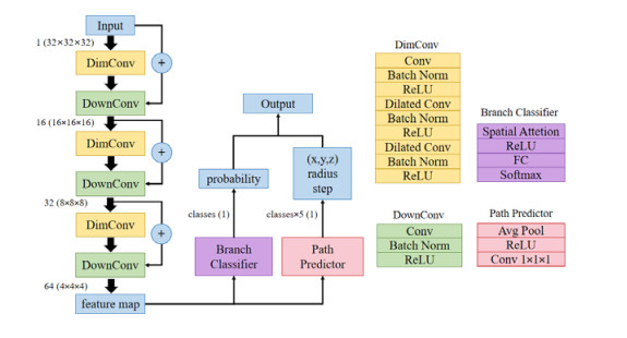
Coronary artery centerline extraction in cardiac computed tomography angiography (CTA) is an effectively non-invasive method to diagnose and evaluate coronary artery disease (CAD). The traditional method of manual centerline extraction is time-consuming and tedious. In this study, we propose a deep learning algorithm that continuously extracts coronary artery centerlines from CTA images using a regression method. In the proposed method, a CNN module is trained to extract the features of CTA images, and then the branch classifier and direction predictor are designed to predict the most possible direction and lumen radius at the given centerline point. Besides, a new loss function is developed for associating the direction vector with the lumen radius. The whole process starts from a point manually placed at the coronary artery ostia, and terminates until tracking the vessel endpoint. The network was trained using a training set consisting of 12 CTA images and the evaluation was performed using a testing set consisting of 6 CTA images. The extracted centerlines had an average overlap (OV) of 89.19%, overlap until first error (OF) of 82.30%, and overlap with clinically relevant vessel (OT) of 91.42% with manually annotated reference. Our proposed method can efficiently deal with multi-branch problems and accurately detect distal coronary arteries, thereby providing potential help in assisting CAD diagnosis.
Citation: Xintong Wu, Yingyi Geng, Xinhong Wang, Jucheng Zhang, Ling Xia. Continuous extraction of coronary artery centerline from cardiac CTA images using a regression-based method[J]. Mathematical Biosciences and Engineering, 2023, 20(3): 4988-5003. doi: 10.3934/mbe.2023231
| [1] | Hüseyin Budak, Abd-Allah Hyder . Enhanced bounds for Riemann-Liouville fractional integrals: Novel variations of Milne inequalities. AIMS Mathematics, 2023, 8(12): 30760-30776. doi: 10.3934/math.20231572 |
| [2] | Muhammad Amer Latif, Humaira Kalsoom, Zareen A. Khan . Hermite-Hadamard-Fejér type fractional inequalities relating to a convex harmonic function and a positive symmetric increasing function. AIMS Mathematics, 2022, 7(3): 4176-4198. doi: 10.3934/math.2022232 |
| [3] | Areej A. Almoneef, Abd-Allah Hyder, Hüseyin Budak, Mohamed A. Barakat . Fractional Milne-type inequalities for twice differentiable functions. AIMS Mathematics, 2024, 9(7): 19771-19785. doi: 10.3934/math.2024965 |
| [4] | Hüseyin Budak, Ebru Pehlivan . Weighted Ostrowski, trapezoid and midpoint type inequalities for RiemannLiouville fractional integrals. AIMS Mathematics, 2020, 5(3): 1960-1984. doi: 10.3934/math.2020131 |
| [5] | Iman Ben Othmane, Lamine Nisse, Thabet Abdeljawad . On Cauchy-type problems with weighted R-L fractional derivatives of a function with respect to another function and comparison theorems. AIMS Mathematics, 2024, 9(6): 14106-14129. doi: 10.3934/math.2024686 |
| [6] | Ghulam Farid, Hafsa Yasmeen, Hijaz Ahmad, Chahn Yong Jung . Riemann-Liouville Fractional integral operators with respect to increasing functions and strongly (α,m)-convex functions. AIMS Mathematics, 2021, 6(10): 11403-11424. doi: 10.3934/math.2021661 |
| [7] | Saad Ihsan Butt, Artion Kashuri, Muhammad Umar, Adnan Aslam, Wei Gao . Hermite-Jensen-Mercer type inequalities via Ψ-Riemann-Liouville k-fractional integrals. AIMS Mathematics, 2020, 5(5): 5193-5220. doi: 10.3934/math.2020334 |
| [8] | Thanin Sitthiwirattham, Muhammad Aamir Ali, Hüseyin Budak, Sotiris K. Ntouyas, Chanon Promsakon . Fractional Ostrowski type inequalities for differentiable harmonically convex functions. AIMS Mathematics, 2022, 7(3): 3939-3958. doi: 10.3934/math.2022217 |
| [9] | Hüseyin Budak, Fatma Ertuğral, Muhammad Aamir Ali, Candan Can Bilişik, Mehmet Zeki Sarikaya, Kamsing Nonlaopon . On generalizations of trapezoid and Bullen type inequalities based on generalized fractional integrals. AIMS Mathematics, 2023, 8(1): 1833-1847. doi: 10.3934/math.2023094 |
| [10] | Abd-Allah Hyder, Hüseyin Budak, Mohamed A. Barakat . Milne-Type inequalities via expanded fractional operators: A comparative study with different types of functions. AIMS Mathematics, 2024, 9(5): 11228-11246. doi: 10.3934/math.2024551 |
Coronary artery centerline extraction in cardiac computed tomography angiography (CTA) is an effectively non-invasive method to diagnose and evaluate coronary artery disease (CAD). The traditional method of manual centerline extraction is time-consuming and tedious. In this study, we propose a deep learning algorithm that continuously extracts coronary artery centerlines from CTA images using a regression method. In the proposed method, a CNN module is trained to extract the features of CTA images, and then the branch classifier and direction predictor are designed to predict the most possible direction and lumen radius at the given centerline point. Besides, a new loss function is developed for associating the direction vector with the lumen radius. The whole process starts from a point manually placed at the coronary artery ostia, and terminates until tracking the vessel endpoint. The network was trained using a training set consisting of 12 CTA images and the evaluation was performed using a testing set consisting of 6 CTA images. The extracted centerlines had an average overlap (OV) of 89.19%, overlap until first error (OF) of 82.30%, and overlap with clinically relevant vessel (OT) of 91.42% with manually annotated reference. Our proposed method can efficiently deal with multi-branch problems and accurately detect distal coronary arteries, thereby providing potential help in assisting CAD diagnosis.
In this paper, we consider the 3D nonlinear damped micropolar equation
| {ut+(u⋅∇)u−(ν+κ)Δu+σ|u|β−1u+∇p=2κ∇×ω+f1(x,t),ωt+(u⋅∇)ω+4κω−γΔω−μ∇∇⋅ω=2κ∇×u+f2(x,t),∇⋅u=0,u(x,t)|t=τ=uτ(x), ω(x,t)|t=τ=ωτ(x), | (1.1) |
where (x,t)∈Ω×[τ,+∞), τ∈R, Ω⊆R3 is a bounded domain, u=u(x,t) is the fluid velocity, ω=ω(x,t) is the angular velocity, σ is the damping coefficient, which is a positive constant, f1=f1(x,t) and f2=f2(x,t) represent external forces, ν, κ, γ, μ are all positive constants, γ and μ represent the angular viscosities.
Micropolar flow can describe a fluid with microstructure, that is, a fluid composed of randomly oriented particles suspended in a viscous medium without considering the deformation of fluid particles. Since Eringen first published his paper on the model equation of micropolar fluids in 1966 [5], the formation of modern theory of micropolar fluid dynamics has experienced more than 40 years of development. For the 2D case, many researchers have discussed the long time behavior of micropolar equations (such as [2,4,10,24]). It should be mentioned that some conclusions in the 2D case no longer hold for the 3D case due to different structures of the system. In the 3D case, the work of micropolar equations (1.1) with σ=0, f1=0, and f2=0 has attracted a lot of attention (see [6,14,19]). Galdi and Rionero [6] proved the existence and uniqueness of solutions of 3D incompressible micropolar equations. In a 3D bounded domain, for small initial data Yamaguchi [19] investigated the existence of a global solution to the initial boundary problem for the micropolar system. In [14], Silva and Cruz et al. studied the L2-decay of weak solutions for 3D micropolar equations in the whole space R3. When f1=f2=0, for the Cauchy problem of the 3D incompressible nonlinear damped micropolar equations, Ye [22] discussed the existence and uniqueness of global strong solutions when β=3 and 4σ(ν+κ)>1 or β>3. In [18], Wang and Long showed that strong solutions exist globally for any 1≤β≤3 when initial data satisfies some certain conditions. Based on [22], Yang and Liu [20] obtained uniform estimates of the solutions for 3D incompressible micropolar equations with damping, and then they proved the existence of global attractors for 3<β<5. In [7], Li and Xiao investigated the large time decay of the L2-norm of weak solutions when β>145, and considered the upper bounds of the derivatives of the strong solution when β>3. In [21], for 1≤β<73, Yang, Liu, and Sun proved the existence of trajectory attractors for 3D nonlinear damped micropolar fluids.
To the best of our knowledge, there are few results on uniform attractors for the three-dimensional micropolar equation with nonlinear damping term. The purpose of this paper is to consider the existence of uniform attractors of system (1.1). When ω=0,κ=0, system (1.1) is reduced to the Navier-Stokes equations with damping. In recent years, some scholars have studied the three-dimensional nonlinear damped Navier-Stokes equations (see [1,13,15,16,23,25]). In order to obtain the desired conclusion, we will use some proof techniques which have been used in the 3D nonlinear damped Navier Stokes equations. Note that, in [20], for the convenience of discussion the authors choose κ,μ=12,γ=1, and ν=32. In this work, we do not specify these parameters, but only require them to be positive real numbers. More importantly, we obtain the existence of uniform attractors in the case of β>3, which undoubtedly expands the range of β when the global attractor exists in [20], i.e., 3<β<5. For the convenience of discussion, similar to [3,8,9,11,16], we make some translational compactness assumption on the external forces term in this paper.
The organizational structure of this article is as follows: In Section 2, we give some basic definitions and properties of function spaces and process theory which will be used in this paper. In Section 3, using various Sobolev inequalities and Gronwall inequalities, we make some uniform estimates from the space with low regularity to high regularity on the solution of the equation. Based on these uniform estimates, in Section 4 we prove that the family of processes {U(f1,f2)(t,τ)}t≥τ corresponding to (1.1) has uniform attractors A1 in V1×V2 and A2 in H2(Ω)×H2(Ω), respectively. Furthermore, we prove A1=A2.
We define the usual functional spaces as follows:
| V1={u∈(C∞0(Ω))3:divu=0,∫Ωudx=0},V2={ω∈(C∞0(Ω))3:∫Ωωdx=0},H1=the closure of V1 in (L2(Ω))3,H2=the closure of V2 in (L2(Ω))3,V1=the closure of V1 in (H1(Ω))3,V2=the closure of V2 in (H1(Ω))3. |
For H1 and H2 we have the inner product
| (u,υ)=∫Ωu⋅υdx, ∀u,v∈H1,or u,v∈H2, |
and norm ‖⋅‖2=‖⋅‖22=(⋅,⋅). In this paper, Lp(Ω)=(Lp(Ω))3, and ‖⋅‖p represents the norm in Lp(Ω).
We define operators
| Au=−PΔu=−Δu, Aω=−Δω, ∀(u,ω)∈H2×H2,B(u)=B(u,u)=P((u⋅∇)u), B(u,ω)=(u⋅∇)ω, ∀(u,ω)∈V1×V2,b(u,υ,ω)=⟨B(u,υ),ω⟩=3∑i,j=1∫Ωui(Diυj)ωjdx, ∀u∈V1,υ,ω∈V2, |
where P is the orthogonal projection from L2(Ω) onto H1. Hs(Ω)=(Hs(Ω))3 is the usual Sobolev space, and its norm is defined by ∥⋅∥Hs=∥As2⋅∥; as s=2, ∥⋅∥H2=∥A⋅∥.
Let us rewrite system (1.1) as
| {ut+B(u)+(ν+κ)Au+G(u)=2κ∇×ω+f1(x,t),ωt+B(u,ω)+4κω+γAω−μ∇∇⋅ω=2κ∇×u+f2(x,t),∇⋅u=0,u(x,t)|t=τ=uτ(x), ω(x,t)|t=τ=ωτ(x), | (2.1) |
where we let G(u)=P(σ|u|β−1u).
The Poincarˊe inequality [17] gives
| √λ1‖u‖≤‖∇u‖,√λ2‖ω‖≤‖∇ω‖,∀(u,ω)∈V1×V2, | (2.2) |
| √λ1∥∇u∥≤∥Au∥, √λ2∥∇ω∥≤∥Aω∥,∀(u,ω)∈H2(Ω)×H2(Ω), | (2.3) |
where λ1 is the first eigenvalue of Au, and λ2 is the first eigenvalue of Aω. Let λ=min{λ1,λ2}. Then, we have
| λ(‖u‖2+‖ω‖2)≤‖∇u‖2+‖∇ω‖2, ∀(u,ω)∈V1×V2,λ(‖∇u‖2+‖∇ω‖2)≤‖Au‖2+‖Aω‖2,∀(u,ω)∈H2(Ω)×H2(Ω). |
Agmon's inequality [17] gives
| ∥u∥∞≤d1∥∇u∥12∥Δu∥12, ∀u∈H2(Ω). |
The trilinear inequalities [12] give
| |b(u,v,w)|≤∥u∥∞∥∇v∥∥w∥,∀u∈L∞(Ω),v∈V1 or V2,w∈H1 or H2, | (2.4) |
| |b(u,v,w)|≤k∥u∥14∥∇u∥34∥∇v∥∥w∥14∥∇w∥34,∀u,v,w∈V1 or V2, | (2.5) |
| |b(u,v,w)|≤k∥∇u∥∥∇v∥12∥Av∥12∥w∥,∀u∈V1 or V2,v∈H2,w∈H1 or H2. | (2.6) |
Recall that a function f(t) is translation bounded (tr.b.) in L2loc(R;L2(Ω)) if
| ∥f∥2L2b=∥f∥2L2b(R;L2(Ω))=supt∈R∫t+1t∥f(t)∥2dt<∞, |
where L2b(R;L2(Ω)) represents the collection of functions that are tr.b. in L2loc(R;L2(Ω)). We say that H(f0)=¯{f0(⋅+t):t∈R} is the shell of f0 in L2loc(R;L2(Ω)). If H(f0) is compact in L2loc(R;L2(Ω)), then we say that f0(x,t)∈L2loc(R;L2(Ω)) is translation compact (tr.c.). We use L2c(R;L2(Ω)) to express the collection of all translation compact functions in L2loc(R;L2(Ω)).
Next, we will provide the existence and uniqueness theorems of the solution of Eq (2.1).
Definition 2.1. A function pair (u,ω) is said to be a global strong solution to system (2.1) if it satisfies
| (u,ω)∈L∞(τ,T;V1×V2)∩L2(τ,T;H2(Ω)×H2(Ω)), |
| |u|β−12∇u∈L2(τ,T;L2(Ω)), ∇|u|β+12∈L2(τ,T;L2(Ω)), |
for any given T>τ.
Theorem 2.1. Suppose (uτ,ωτ)∈V1×V2 with ∇⋅uτ=0,f1,f2∈L2b(R;L2(Ω)). If β=3 and 4σ(ν+κ)>1 or β>3, then there exists a unique global strong solution of (2.1).
Proof. Since the proof method is similar to that of Theorem 1.2 in [22], we omit it here.
Let Σ be a metric space. X, Y are two Banach spaces, and Y⊂X is continuous. {Uσ(t,τ)}t≥τ, σ∈Σ is a family of processes in Banach space X, i.e., u(t)=Uσ(t,τ)uτ, Uσ(t,s)Uσ(s,τ)=Uσ(t,τ),∀t≥s≥τ,τ∈R,Uσ(τ,τ)=I, where σ∈Σ is a time symbol space. B(X) is the set of all bounded subsets of X. Rτ=[τ,+∞).
For the basic concepts of bi-space uniform absorbing set, uniform attracting set, uniform attractor, uniform compact, and uniform asymptotically compact of the family of processed {Uσ(t,τ)}t≥τ,σ∈Σ, one can refer to [9,16].
Let T(h) be a family of operators acting on Σ, satisfying: T(h)σ(s)=σ(s+h),∀s∈R. In this paper, we assume that Σ satisfies
(C1) T(h)Σ=Σ, ∀h∈R+;
(C2) translation identity:
| Uσ(t+h,τ+h)=UT(h)σ(t,τ), ∀σ∈Σ,t≥τ,τ∈R,h≥0. |
Theorem 2.2. [3] If the family of processes {Uσ(t,τ)}t≥τ,σ∈Σ is (X,Y)-uniformly (w.r.t. σ∈Σ) asymptotically compact, then it has a (X,Y)-uniform (w.r.t. σ∈Σ) attractor AΣ, AΣ is compact in Y, and it attracts all bounded subsets of X in the topology of Y.
In this paper, the letter C represents a positive constant. It may represent different values in different lines, or even in the same line.
In this paper, we chose H(f01)×H(f02) as the symbol space. Obviously, T(t)(H((f01)×H(f02))=H(f01)×H(f02), for all t≥0. {T(t)}t≥0 is defined by
| T(h)(f1(⋅),f2(⋅))=(f1(⋅+h),f2(⋅+h)), ∀h≥0,(f1,f2)∈H(f01)×H(f02), |
which is a translation semigroup and is continuous on H(f01)×H(f02).
Thanks to Theorem 2.1, when (uτ,ωτ)∈V1×V2, f1,f2∈L2loc(R;L2(Ω)), and β>3, we can define a process {U(f1,f2)(t,τ)}t≥τ in V1×V2 by
| U(f1,f2)(t,τ)(uτ,ωτ)=(u(t),ω(t)), t≥τ, |
where (u(t),ω(t)) is the solution of Eq (1.1) with external forces f1,f2 and initial data (uτ,ωτ).
Next, let us assume that the external forces f01(x,t),f02(x,t) are tr.c. in L2loc(R;L2(Ω)). Then, f01,f02 are tr.b. in L2loc(R;L2(Ω)), and
| ∥f1∥2L2b=∥f1∥2L2b(R;L2(Ω))=supt∈R∫t+1t∥f1(s)∥2ds≤∥f01∥2L2b<+∞,∀f1∈H(f01), |
| ∥f2∥2L2b=∥f2∥2L2b(R;L2(Ω))=supt∈R∫t+1t∥f2(s)∥2ds≤∥f02∥2L2b<+∞,∀f2∈H(f02). |
Furthermore, we assume f01,f02 are uniformly bounded in L2(Ω), i.e., there exists a positive constant K, which satisfies
| supt∈R∥f01(x,t)∥≤K, supt∈R∥f02(x,t)∥≤K. |
Meanwhile, we suppose the derivatives df01dt, df02dt, labeled as h1,h2, also belong to L2c(R;L2(Ω)).
Lemma 3.1. Suppose (uτ,ωτ)∈V1×V2 and (f1,f2)∈H(f01)×H(f02). If β>3 then there exists a time t0 and constants ρ1,I1 such that, for any t≥t0,
| ‖u(t)‖2+‖ω(t)‖2≤ρ1, | (3.1) |
| ∫t+1t[‖∇u(s)‖2+‖∇ω(s)‖2+‖u(s)‖β+1β+1+‖∇⋅ω(s)‖2]ds≤I1. | (3.2) |
Proof. Multiplying (1.1)1 and (1.1)2 with external forces f1∈H(f01), f2∈H(f02) by u and ω, respectively, and integrating the results equations on Ω, using H¨older's inequality, Young's inequality, and Poincarˊe's inequality, it yields
| 12ddt(‖u(t)‖2+‖ω(t)‖2)+(ν+κ)‖∇u‖2+γ‖∇ω‖2+4κ‖ω(t)‖2+σ‖u(t)‖β+1β+1+μ‖∇⋅ω‖2=4κ∫Ω∇×u⋅ωdx+(f1,u(t))+(f2,ω(t))≤κ∥∇u∥2+4κ∥ω∥2+νλ2∥u∥2+γλ2∥ω∥2+12νλ∥f1∥2+12γλ∥f2∥2≤(ν2+κ)‖∇u‖2+γ2‖∇ω‖2+4κ‖ω(t)‖2+12νλ∥f1∥2+12γλ∥f2∥2. | (3.3) |
So, we can obtain that
| ddt(‖u(t)‖2+‖ω(t)‖2)+ν‖∇u‖2+γ‖∇ω‖2+2σ‖u(t)‖β+1β+1+2μ‖∇⋅ω‖2≤1νλ‖f1(t)‖2+1γλ‖f2(t)‖2, | (3.4) |
and by Poincarˊe's inequality, it yields
| ddt(‖u(t)‖2+‖ω(t)‖2)+λα(‖u(t)‖2+‖ω(t)‖2)≤1λα(‖f1(t)‖2+‖f2(t)‖2), | (3.5) |
where α=min{ν,γ}. So, by Gronwall's inequality, we get
| ‖u(t)‖2+‖ω(t)‖2≤(‖uτ‖2+‖ωτ‖2)e−λα(t−τ)+1λα∫tτe−λα(t−s)(‖f1(s)‖2+‖f2(s)‖2)ds≤(‖uτ‖2+‖ωτ‖2)e−λα(t−τ)+1λα[∫tt−1e−λα(t−s)(‖f1(s)‖2+‖f2(s)‖2)ds+∫t−1t−2e−λα(t−s)(‖f1(s)‖2+‖f2(s)‖2)ds+...]≤(‖uτ‖2+‖ωτ‖2)e−λα(t−τ)+1λα[1+e−λα+e−2λα+...](‖f1‖2L2b+‖f2‖2L2b)≤(‖uτ‖2+‖ωτ‖2)e−λα(t−τ)+1λα(1−e−λα)−1(‖f1‖2L2b+‖f2‖2L2b)≤(‖uτ‖2+‖ωτ‖2)e−λα(t−τ)+1λα(1+1λα)(‖f1‖2L2b+‖f2‖2L2b), ∀t≥τ. |
Therefore, there must exists a time t0≥τ+1λαlnλ2α2(‖uτ‖2+‖ωτ‖2)(1+λα)(‖f1‖2L2b+‖f2‖2L2b), such that, ∀t≥t0,
| ‖u(t)‖2+‖ω(t)‖2≤2λα(1+1λα)(‖f1‖2L2b+‖f2‖2L2b)≡ρ1. | (3.6) |
Taking t≥t0, integrating (3.4) from t to t+1, and noticing (3.6), we get
| ∫t+1t[ν‖∇u(s)‖2+γ‖∇ω(s)‖2+2σ‖u(s)‖β+1β+1+2μ‖∇⋅ω(s)‖2]ds≤(‖u(t)‖2+‖ω(t)‖2)+1νλ∫t+1t‖f1(s)‖2ds+1γλ∫t+1t‖f2(s)‖2ds≤ρ1+1λα(‖f1‖2L2b+‖f2‖2L2b), ∀t≥t0. | (3.7) |
Letting δ1=min{ν,γ,2σ,2μ}, we have
| δ1∫t+1t[‖∇u(s)‖2+‖∇ω(s)‖2+‖u(s)‖β+1β+1+‖∇⋅ω(s)‖2]ds≤ρ1+1λα(‖f1‖2L2b+‖f2‖2L2b), ∀t≥t0. |
Letting I1=1δ1(ρ1+1λα(‖f1‖2L2b+‖f2‖2L2b)), we have
| ∫t+1t[‖∇u(s)‖2+‖∇ω(s)‖2+‖u(s)‖β+1β+1+‖∇⋅ω(s)‖2]ds≤I1, ∀t≥t0. |
This completes the proof of Lemma 3.1.
Lemma 3.2. Assume β>3, (uτ,ωτ)∈V1×V2 and (f1,f2)∈H(f01)×H(f02). Then, there exists a time t2 and a constant ρ2 such that
| ‖∇u(t)‖2+‖∇ω(t)‖2+∫t+1t(‖Au(s)‖2+‖Aω(s)‖2+‖|u|β−12∇u‖2+‖∇|u|β+12‖2)ds≤ρ2, | (3.8) |
for any t≥t2.
Proof. Taking the inner product of −Δu in H1 with the first equation of (1.1), we obtain
| 12ddt‖∇u‖2+(ν+κ)‖Au‖2+σ‖|u|β−12∇u‖2+4σ(β−1)(β+1)2‖∇|u|β+12‖2=−b(u,u,Au)+2κ∫Ω∇×ω⋅Audx+(f1(t),Au). | (3.9) |
In [18], we find that, when β>3,
| ∫Ω(u⋅∇u)⋅Δudx≤ν+κ4∥Δu∥2+σ2∥|u|β−12∇u∥2+C1∥∇u∥2, | (3.10) |
where C1=N2ν+κ+N2(ν+κ)(Nβ−1+1), and N is sufficiently large such that
| N≥(2β−3)1β−1 and N2(ν+κ)(Nβ−1+1)≤σ2. |
And, because
| |2κ∫Ω∇×ω⋅Audx|≤ν+κ4∥Δu∥2+4κ2ν+κ∥∇ω∥2, | (3.11) |
| |(f1(t),Au)|≤ν+κ4∥Δu∥2+∥f1(t)∥2ν+κ, | (3.12) |
so combining (3.10)–(3.12) with (3.9), we have
| ddt‖∇u‖2+ν+κ2‖Au‖2+σ‖|u|β−12∇u‖2+8σ(β−1)(β+1)2‖∇|u|β+12‖2≤2C1‖∇u‖2+8κ2ν+κ∥∇ω∥2+2∥f1(t)∥2ν+κ≤C2(‖∇u‖2+‖∇ω‖2+‖f1(t)‖2), | (3.13) |
where C2=max{2C1,8κ2ν+κ,2ν+κ}.
Applying uniform Gronwall's inequality to (3.13), we obtaint, ∀t≥t0+1≡t1,
| ‖∇u(t)‖2+∫t+1t(ν+κ2‖Au(s)‖2+σ‖|u(s)|β−12∇u(s)‖2+8σ(β−1)(β+1)2‖∇|u(s)|β+12‖2)ds≤C3, | (3.14) |
where C3 is a positive constant dependent on C2, I1, and ∥f01∥2L2b.
Taking the inner product of −Δω in H2 with the second equation of (1.1), we get
| 12ddt‖∇ω‖2+4κ‖∇ω‖2+γ‖Aω‖2+μ‖∇∇⋅ω‖2=−b(u,ω,Aω)+2κ∫Ω∇×u⋅Aωdx+(f2(t),Aω)≤3γ4‖Aω‖2+d21γ‖∇u‖‖Au‖‖∇ω‖2+4κ2γ‖∇u‖2+1γ‖f2(t)‖2. | (3.15) |
In the last inequality of (3.15), we used Agmon's inequality and the trilinear inequality. Then,
| ddt‖∇ω‖2+γ2‖Aω‖2+2μ‖∇∇⋅ω‖2≤C4(‖∇u‖‖Au‖‖∇ω‖2+‖∇u‖2+‖f2(t)‖2), | (3.16) |
where C4=max{2d21γ,8κ2γ,2γ}.
By the uniform Gronwall's inequality, we easily obtain that, for t≥t1+1≡t2,
| ‖∇ω(t)‖2+∫t+1t(γ2‖Aω(s)‖2+2μ‖∇∇⋅ω(s)‖2)ds≤C5, for t≥t1+1≡t2, | (3.17) |
where C5 is a positive constant dependent on C3,C4, and ∥f02∥2L2b.
Adding (3.14) with (3.17) yields
| ‖∇u(s)‖2+‖∇ω(s)‖2+∫t+1t(‖Au(s)‖2+‖Aω(s)‖2+‖|u(s)|β−12∇u(s)‖2+‖∇|u(s)|β+12‖2)ds≤C, |
for t≥t2. Hence, Lemma 3.2 is proved.
Lemma 3.3. Suppose that (uτ,ωτ)∈V1×V2 and (f1,f2)∈H(f01)×H(f02). Then, for β>3, there exists a time t3 and a constant ρ3 such that
| ‖u(t)‖β+1+‖∇⋅ω(t)‖2≤ρ3, | (3.18) |
for any t≥t3.
Proof. Multiplying (1.1)1 by ut, then integrating the equation over Ω, we have
| ‖ut‖2+ν+κ2ddt‖∇u‖2+σβ+1ddt‖u(t)‖β+1β+1=−b(u,u,ut)+2κ∫Ω∇×ω⋅utdx+(f1(t),ut)≤12‖ut‖2+3d212√λ1∥∇u∥2∥Au∥2+6κ2‖∇ω‖2+32‖f1(t)‖2. | (3.19) |
The trilinear inequality (2.4), Agmon's inequality, and Poincarˊe's inequality are used in the last inequality of (3.19).
Hence,
| (ν+κ)ddt‖∇u‖2+2σβ+1ddt‖u(t)‖β+1β+1≤C6(∥∇u∥2∥Au∥2+‖∇ω‖2+‖f1(t)‖2), | (3.20) |
where C6=max{3d21√λ1,12κ2,3}.
By (3.20), using Lemmas 3.1 and 3.2 and the uniform Gronwall's inequality, we have
| ‖u(t)‖β+1≤C, ∀t≥t2+1≡t3. | (3.21) |
Similar to (3.19), multiplying (1.1)2 by ωt and integrating it over Ω, we get
| ‖ωt‖2+2κddt‖ω‖2+γ2ddt‖∇ω‖2+μ2ddt‖∇⋅ω‖2=−b(u,ω,ωt)+2κ∫Ω∇×u⋅ωtdx+(f2(t),ωt)≤12‖ωt‖2+3d212√λ1∥Au∥2∥∇ω∥2+6κ2‖∇u‖2+32‖f2(t)‖2. | (3.22) |
Hence,
| 4κddt∥ω∥2+γddt∥∇ω∥2+μddt∥∇⋅ω∥2≤C6(∥Au∥2∥∇ω∥2+∥∇u∥2+∥f2(t)∥2). | (3.23) |
By (3.23), using Lemma 3.2 and the uniform Gronwall's inequality, we infer that
| ‖∇⋅ω(t)‖2≤C, ∀t≥t3. | (3.24) |
The proof of Lemma 3.3 is finished.
Lemma 3.4. Suppose (uτ,ωτ)∈V1×V2 and (f1,f2)∈H(f01)×H(f02). If β>3, then there exists a time t4 and a constant ρ5, such that
| ‖ut(s)‖2+‖ωt(s)‖2≤ρ5, | (3.25) |
for any s≥t4.
Proof. Taking the inner products of ut and ωt with the first and second equations of (1.1), respectively, and using (3.19) and (3.22), we find
| ‖ut‖2+‖ωt‖2+ν+κ2ddt‖∇u‖2+γ2ddt‖∇ω‖2+2κddt‖ω(t)‖2+σβ+1ddt‖u(t)‖β+1β+1+μ2ddt‖∇⋅ω‖2=−b(u,u,ut)−b(u,ω,ωt)+2κ∫Ω∇×ω⋅utdx+2κ∫Ω∇×u⋅ωtdx+(f1(t),ut)+(f2(t),ωt)≤12(‖ut‖2+‖ωt‖2)+C7(‖f1(t)‖2+‖f2(t)‖2+‖∇u‖2+‖∇ω‖2+∥∇u∥2∥Au∥2+∥∇ω∥2∥Au∥2), | (3.26) |
where C7=max{3d212√λ1,6κ2,32}. The trilinear inequality (2.4), Agmon's inequality, and Poincarˊe's inequality are used in the last inequality of (3.26).
Integrating (3.26) over [t,t+1] and using Lemmas 3.1–3.3, we get
| ∫t+1t(‖ut(s)‖2+‖ωt(s)‖2)ds≤ρ4, ∀t≥t3, | (3.27) |
where ρ4 is a positive constant dependent on C7,ρ2,ρ3, ∥f01∥2L2b, and ∥f02∥2L2b.
We now differentiate (2.1)1 with respect to t, then take the inner product of ut with the resulting equation to obtain
| 12ddt∥ut∥2+(ν+κ)∥∇ut∥2=−b(ut,u,ut)−∫ΩG′(u)ut⋅utdx+2κ∫Ω∇×ωt⋅utdx+(f1t,ut). | (3.28) |
Then, we differentiate (2.1)2 with respect to t and take the inner product with ωt to obtain
| 12ddt∥ωt∥2+4κ∥ωt∥2+γ∥∇ωt∥2+μ∥∇⋅ωt∥2=−b(ut,ω,ωt)+2κ∫Ω∇×ut⋅ωtdx+(f2t,ωt). | (3.29) |
Adding (3.28) with (3.29), we have
| 12ddt(‖ut‖2+‖ωt‖2)+(ν+κ)‖∇ut‖2+γ‖∇ωt‖2+4κ‖ωt‖2+μ‖∇⋅ωt‖2≤|b(ut,u,ut)|+|b(ut,ω,ωt)|+2κ∫Ω∇×ωt⋅utdx+2κ∫Ω∇×ut⋅ωtdx+(f1t,ut)+(f2t,ωt)−∫ΩG′(u)ut⋅utdx:=7∑i=1Li. | (3.30) |
From Lemma 2.4 in [15], we know that G′(u) is positive definite, so
| L7=−∫ΩG′(u)ut⋅utdx≤0. | (3.31) |
For L1, using the trilinear inequality (2.5) and Lemma 3.2, we have
| L1≤k‖ut‖12‖∇ut‖32‖∇u‖≤ν+κ4‖∇ut‖2+C‖ut‖2‖∇u‖4≤ν+κ4‖∇ut‖2+C‖ut‖2, for t≥t2. | (3.32) |
For L2, by H¨older's inequality, Gagliardo-Nirenberg's inequality, and Young's inequality, we have
| L2≤C‖ut‖4‖ωt‖4‖∇ω‖≤C‖ut‖14‖∇ut‖34‖ωt‖14‖∇ωt‖34‖∇ω‖≤ν+κ4‖∇ut‖2+γ4‖∇ωt‖2+C(‖ut‖2+‖ωt‖2), for t≥t2. | (3.33) |
| L3+L4≤ν+κ4‖∇ut‖2+γ2‖∇ωt‖2+C(‖ut‖2+‖ωt‖2). | (3.34) |
By (3.30)–(3.34), we get
| ddt(‖ut‖2+‖ωt‖2)≤C(‖ut‖2+‖ωt‖2)+(f1t,ut)+(f2t,ωt)≤C(‖ut‖2+‖ωt‖2)+‖f1t‖2+‖f2t‖2. | (3.35) |
Thanks to
| ∫t+1t∥f1t(s)∥2ds≤∥f1t∥2L2b≤∥h1∥2L2b,∫t+1t∥f2t(s)∥2ds≤∥f2t∥2L2b≤∥h2∥2L2b, |
and applying uniform Gronwall's inequality to (3.35), we have for any s≥t3+1≡t4,
| ‖ut(s)‖2+‖ωt(s)‖2≤C. | (3.36) |
Thus, Lemma 3.4 is proved.
Lemma 3.5. Suppose (uτ,ωτ)∈V1×V2 and (f1,f2)∈H(f01)×H(f02). Then, for β>3, there exists a constant ρ6 such that
| ‖Au(t)‖2+‖Aω(t)‖2≤ρ6, | (3.37) |
for any t≥t4.
Proof. Taking the inner product of −Δu in H1 with the first equation of (1.1), we have
| (ν+κ)∥Au∥2+σ∥|u|β−12∇u∥2+4σ(β−1)(β+1)2∥∇|u|β+12∥2=−(ut,Au)−(B(u),Au)+2κ∫Ω∇×ω⋅Audx+(f1(t),Au)≤4(ν+κ)6∥Au∥2+32(ν+κ)∥ut∥2+32(ν+κ)∥B(u)∥2+6κ2ν+κ∥∇ω∥2+32(ν+κ)∥f1(t)∥2. | (3.38) |
Because
| \begin{align} \frac{3}{2(\nu+\kappa)}\parallel B(u)\parallel^2&\leq\frac{3}{2(\nu+\kappa)}\parallel u\parallel_\infty^2\parallel\nabla u\parallel^2\\ &\leq \frac{3d_1^2}{2(\nu+\kappa)}\parallel\nabla u\parallel^3\parallel\Delta u\parallel\\ &\leq\frac{\nu+\kappa}{6}\parallel Au\parallel^2+C\parallel\nabla u\parallel^6, \end{align} | (3.39) |
combining (3.39) with (3.38), we obtain
| \begin{equation} \frac{\nu+\kappa}{6}\parallel Au\parallel^2\leq \frac{3}{2(\nu+\kappa)}\parallel u_t\parallel^2+C\parallel\nabla u\parallel^6+\frac{6\kappa^2}{\nu+\kappa}\parallel\nabla\omega\parallel^2+\frac{3}{2(\nu+\kappa)}\parallel f_1(t)\parallel^2. \end{equation} | (3.40) |
From the assumption of f_1^0(t) , we can easily get
| \begin{equation} \sup\limits_{t\in\mathbb{R}}\parallel f_1(t)\parallel\leq\sup\limits_{t\in\mathbb{R}}\parallel f_{1}^0(t)\parallel\leq K, \forall f_1\in\mathcal{H}(f_1^0). \end{equation} | (3.41) |
By Lemmas 3.2 and 3.4, we obtain
| \begin{eqnarray} \|Au(t)\|\leq C,\ \text{for any}\ t\geq t_4. \end{eqnarray} | (3.42) |
Taking the inner product of A\omega with (2.1)_{2} , we get
| \begin{align} &\quad\gamma\|A\omega\|^{2}+4\kappa\parallel\nabla \omega\parallel^2+\mu\parallel\nabla\nabla\cdot\omega\parallel^2\\ & = -(\omega_t,A\omega)-(B(u,\omega),A\omega)+2\kappa(\nabla\times u,A\omega)+(f_2(t),A\omega)\\ &\leq\frac{\gamma}{2}\parallel A\omega\parallel^2+C(\parallel \omega_t\parallel^2+\parallel B(u,\omega)\parallel^2+\parallel\nabla u\parallel^2+\parallel f_2(t)\parallel^2). \end{align} | (3.43) |
And, by Agmon's inequality,
| \begin{align} \|B(u,\omega)\|^2&\leq C\|u\|_{\infty}^2\|\nabla \omega\|^2\\ &\leq C\|\nabla u\|\|\Delta u\|\|\nabla\omega\|^2\\ &\leq\|Au\|^2+C\parallel\nabla u\parallel^2\parallel\nabla\omega\parallel^4. \end{align} | (3.44) |
From the assumption on f_2^0(t) , we can easily obtain
| \begin{equation} \sup\limits_{t\in\mathbb{R}}\parallel f_2(t)\parallel\leq\sup\limits_{t\in\mathbb{R}}\parallel f_{2}^0(t)\parallel\leq K, \forall f_2\in\mathcal{H}(f_2^0). \end{equation} | (3.45) |
By Lemma 3.2, Lemma 3.4, (3.42), (3.43), (3.44), and (3.45), we get
| \begin{eqnarray} \|A\omega(t)\|\leq C,\ \text{for any }t\geq t_{4}. \end{eqnarray} | (3.46) |
By (3.42) and (3.46), Lemma 3.5 is proved for all t\geq t_{4} .
Lemma 3.6. Suppose (u_{\tau}, \omega_{\tau})\in V_{1}\times V_{2} and (f_{1}, f_{2})\in \mathcal{H}(f_{1}^{0})\times \mathcal{H}(f_{2}^{0}) . Then, for \beta > 3 , there exists a time t_5 and a constant \rho_{7} satisfying
| \begin{eqnarray} \|\nabla u_{t}(t)\|^{2}+\|\nabla\omega_{t}(t)\|^{2}\leq \rho_7, \forall t\geq t_{5}. \end{eqnarray} | (3.47) |
Proof. In the proof of Lemma 3.4, from (3.30)–(3.34) we can also get
| \begin{align} &\quad\frac{d}{dt}(\parallel u_t\parallel^2+\parallel\omega_t\parallel^2)+\frac{\nu+\kappa}{2}\parallel\nabla u_t\parallel^2+\frac{\gamma}{2}\parallel\nabla\omega_t\parallel^2+2\mu\parallel \nabla\cdot\omega_t\parallel^2\\ &\leq C(\parallel u_t\parallel^2+\parallel\omega_t\parallel^2)+\parallel f_1(t)\parallel^2+\parallel f_2(t)\parallel^2. \end{align} | (3.48) |
Integrating (3.48) from t to t+1 , and according to Lemma 3.4, we have
| \begin{align} &\quad\int^{t+1}_{t}(\|\nabla u_{t}(s)\|^{2}+\|\nabla\omega_{t}(s)\|^{2}+\|\nabla\cdot\omega_{t}(s)\|^{2})ds\\ &\leq C(\|u_{t}(t)\|^{2}+\|\omega_{t}(t)\|^{2}+\int^{t+1}_{t}(\|u_{t}(s)\|^{2}+\|\omega_{t}(s)\|^{2})ds+\int^{t+1}_{t}\|f_{1t}(s)\|^{2}ds+\int^{t+1}_{t}\|f_{2t}(s)\|^{2}ds)\\ &\leq C+\|h_{1}\|^{2}_{L^{2}_{b}}+\|h_{2}\|^{2}_{L^{2}_{b}}\\ &\leq C,\ \forall t\geq t_4. \end{align} | (3.49) |
By Lemma 3.5, we get
| \begin{eqnarray} \|u(t)\|_{H^{2}}+\|\omega(t)\|_{H^{2}}\leq C, \forall t\geq t_4. \end{eqnarray} | (3.50) |
So, by Lemma 3.2, applying Agmon's inequality, we get
| \begin{eqnarray} \|u(t)\|_{\infty}+\|\omega(t)\|_{\infty}\leq C, \forall t\geq t_4. \end{eqnarray} | (3.51) |
Taking the derivative of (2.1)_{1} and (2.1)_{2} with respect to t , then multiplying by Au_{t} and A\omega_{t} , respectively, and integrating the resulting equations over \Omega , we then have
| \begin{align} &\quad\frac{1}{2}\frac{d}{dt}(\|\nabla u_{t}\|^{2}+\|\nabla\omega_{t}\|^{2})+(\nu+\kappa)\|Au_{t}\|^{2}+\gamma\|A\omega_{t}\|^{2}+4\kappa\|\nabla\omega_{t}\|^{2}+\mu\parallel\nabla\nabla\cdot\omega_t\parallel^2\\ &\leq|b(u_t,u,Au_t)|+|b(u,u_{t},Au_{t})|+|b(u,\omega_{t},A\omega_{t})|+|b(u_{t},\omega,A\omega_{t})|\\ &\ \ \ \ +2\kappa\int_{\Omega}|\nabla\times\omega_{t}\cdot Au_{t}|dx+2\kappa\int_{\Omega}|\nabla\times u_{t}\cdot A\omega_{t}|dx+|\int_{\Omega}G'(u)u_{t}\cdot Au_{t}dx|\\ &\ \ \ \ +(f_{1t},Au_{t})+(f_{2t},A\omega_{t})\\ &: = \sum^{9}_{i = 1}J_{i}. \end{align} | (3.52) |
For J_{1} , J_2 , using (2.6) and Lemmas 3.2 and 3.5, we have
| \begin{align} J_{1}&\leq k\|\nabla u_{t}\|\|\nabla u\|^{\frac{1}{2}}\|Au\|^{\frac{1}{2}}\|Au_{t}\|\\ &\leq\frac{\nu+\kappa}{5}\|Au_{t}\|^{2}+C\|\nabla u_{t}\|^{2},\ \forall t\geq t_4, \end{align} | (3.53) |
and
| \begin{align} J_{2}&\leq k\|\nabla u\|\|\nabla u_{t}\|^{\frac{1}{2}}\|A u_{t}\|^{\frac{1}{2}}\|Au_{t}\|\\ &\leq k\|\nabla u\|\|\nabla u_{t}\|^{\frac{1}{2}}\|Au_{t}\|^{\frac{3}{2}}\\ &\leq \frac{\nu+\kappa}{5}\|Au_{t}\|^{2}+C\|\nabla u_{t}\|^{2},\ \forall t\geq t_4. \end{align} | (3.54) |
For J_{3} and J_{4} , similar to (3.53) and (3.54), we get
| \begin{align} J_{3}&\leq k\|\nabla u\|\|\nabla\omega_t\|^{\frac{1}{2}}\|A\omega_{t}\|^{\frac{1}{2}}\|A\omega_{t}\|\\ &\leq \frac{\gamma}{4}\|A\omega_{t}\|^{2}+C\|\nabla \omega_{t}\|^{2},\ \forall t\geq t_4, \end{align} | (3.55) |
| \begin{align} J_{4}&\leq k\|\nabla u_{t}\|\|\nabla\omega\|^{\frac{1}{2}}\|A\omega\|^{\frac{1}{2}}\|A\omega_{t}\|\\ &\leq\frac{\gamma}{4}\|A\omega_{t}\|^{2}+C\|\nabla u_{t}\|^{2},\ \forall t\geq t_4. \end{align} | (3.56) |
For J_{5} , J_6 , and J_{7} , applying Hölder's inequality and Young's inequality, we have
| \begin{align} J_{5}+J_{6}\leq\frac{\nu+\kappa}{5}\|Au_{t}\|^{2}+\frac{\gamma}{4}\|A\omega_{t}\|^{2}+C(\|\nabla u_{t}\|^{2}+\|\nabla\omega_{t}\|^{2}), \end{align} | (3.57) |
and thanks to (3.51),
| \begin{align} J_{7}&\leq C\|u\| ^{\beta-1}_{\infty}\|u_{t}\|\|Au_{t}\|\\ &\leq\frac{\nu+\kappa}{5}\|Au_{t}\|^{2}+C\|u_{t}\|^{2},\ \forall t\geq t_4. \end{align} | (3.58) |
For J_8 and J_9 , we have
| \begin{align} J_{8}&\leq\frac{\nu+\kappa}{5}\|Au_{t}\|^{2}+C\|f_{1t}\|^{2}, \end{align} | (3.59) |
| \begin{align} J_{9}&\leq\frac{\gamma}{4}\|A\omega_{t}\|^{2}+C\|f_{2t}\|^{2}. \end{align} | (3.60) |
By (3.52)–(3.60), we obtain
| \begin{eqnarray} \frac{d}{dt}(\|\nabla u_{t}\|^{2}+\|\nabla\omega_{t}\|^{2})\leq C(\|\nabla u_{t}\|^{2}+\|\nabla\omega_{t}\|^{2})+C\|u_{t}\|^{2}+C(\|f_{1t}\|^{2}+\|f_{2t}\|^{2}). \end{eqnarray} | (3.61) |
Then, by (3.27), (3.49), and using the uniform Gronwall's lemma, we get
| \begin{eqnarray} \|\nabla u_{t}(s)\|^{2}+\|\nabla\omega_{t}(s)\|^{2}\leq C,\ \forall s\geq t_{4}+1\equiv t_{5}. \end{eqnarray} | (3.62) |
Thus, Lemma 3.6 is proved.
In this section, we consider the existence of the (V_1\times V_2, V_1\times V_2) -uniform (w.r.t. (f_1, f_2)\in \mathcal{H}(f_1^0)\times\mathcal{H}(f_2^0) ) attractor and the (V_1\times V_2, \mathbf{H}^2(\Omega)\times \mathbf{H}^2(\Omega)) -uniform attractor for \{U_{(f_1, f_2)}(t, \tau)\}_{t\geq\tau}, f_1\times f_2\in \mathcal{H}(f^{0}_{1})\times \mathcal{H}(f^{0}_{2}) .
Lemma 4.1. Suppose \beta > 3 . The family of processes \{U_{(f_{1}, f_{2})}(t, \tau)\}_{t\geq\tau} , f_{1}\times f_{2}\in\mathcal{H}(f^{0}_{1})\times \mathcal{H}(f^{0}_{2}) , corresponding to (2.1) is ((V_{1}\times V_{2})\times(\mathcal{H}(f^{0}_{1})\times \mathcal{H}(f^{0}_{2})), V_{1}\times V_{2}) -continuous for \tau\geq t_5.
Proof. Let \tau_n\subset [\tau, +\infty) be a time sequence, U_{(f_{1}^{(n)}, f_{2}^{(n)})}(t, \tau)(u_{\tau_n}, \omega_{\tau_n}) = (u^{(n)}(t), \omega^{(n)}(t)) , U_{(f_{1}, f_{2})}(t, \tau)(u_{\tau}, \omega_{\tau}) = (u(t), \omega(t)) and
| \begin{align*} (\bar{u}^{(n)}(t),\bar{\omega}^{(n)}(t))& = (u(t)-u^{(n)}(t),\omega(t)-\omega^{(n)}(t))\\ & = U_{(f_{1},f_{2})}(t,\tau)(u_{\tau},\omega_{\tau})-U_{(f_{1}^{(n)},f_{2}^{(n)})}(t,\tau)(u_{\tau_n},\omega_{\tau_n}). \end{align*} |
It is evident that \bar{u}^{(n)}(t) is the solution of
| \begin{align} \frac{\partial\bar{u}^{(n)}(t)}{\partial t}+B(u)-B(u^{(n)}(t))+(\nu+\kappa)A\bar{u}^{(n)}+G(u)-G(u^{(n)}) = 2\kappa\nabla\times\bar{\omega}^{(n)}+(f_{1}-f_{1}^{(n)}), \end{align} | (4.1) |
and \bar{\omega}^{(n)}(t) is the solution of the following system
| \begin{align} \frac{\partial\bar{\omega}^{(n)}(t)}{\partial t}&+B(u,\omega)-B(u^{(n)},\omega^{(n)})+4\kappa\bar{\omega}^{(n)}+\gamma A\bar{\omega}^{(n)}-\mu\nabla\nabla\cdot\bar{\omega}^{(n)} = 2\kappa\nabla\times\bar{u}^{(n)}+(f_{2}-f_{2}^{(n)}), \end{align} | (4.2) |
for each n .
Taking the inner product of (4.1) with A\bar{u}^{(n)} in H_1 , we get
| \begin{align} &\quad\frac{1}{2}\frac{d}{dt}\|\nabla\bar{u}^{(n)}\|^{2}+b(u,u,A\bar{u}^{(n)})-b(u^{(n)},u^{(n)},A\bar{u}^{(n)}) +(\nu+\kappa)\parallel A\bar{u}^{(n)}\parallel^2+(G(u)-G(u^{(n)}),A\bar{u}^{(n)})\\& = 2\kappa(\nabla\times\bar{\omega}^{(n)},A\bar{u}^{(n)})+(f_{1}-f_{1}^{(n)},A\bar{u}^{(n)}). \end{align} | (4.3) |
Taking the inner product of (4.2) with A\bar{\omega}^{(n)} in H_2 , we have
| \begin{align} &\quad\frac{1}{2}\frac{d}{dt}\|\nabla\bar{\omega}^{(n)}\|^{2}+b(u,\omega,A\bar{\omega}^{(n)})-b(u^{(n)},\omega^{(n)},A\bar{\omega}^{(n)}) +4\kappa\|\nabla\bar{\omega}^{(n)}\|^2+\gamma\parallel A\bar{\omega}^{(n)}\parallel^2+\mu\parallel\nabla\nabla\cdot\bar{\omega}^{(n)}\parallel^2\\ & = 2\kappa(\nabla\times\bar{u}^{(n)},A\bar{\omega}^{(n)})+(f_{2}-f_{2}^{(n)},A\bar{\omega}^{(n)}). \end{align} | (4.4) |
Combining (4.3) with (4.4), we get
| \begin{align} &\quad\frac{1}{2}\frac{d}{dt}(\|\nabla\bar{u}^{(n)}\|^{2}+\|\nabla\bar{\omega}^{(n)}\|^{2})+b(u,u,A\bar{u}^{(n)})-b(u^{(n)},u^{(n)},A\bar{u}^{(n)})+(\nu+\kappa)\|A\bar{u}^{(n)}\|^{2}\\ &\quad+(G(u)-G(u^{(n)}),A\bar{u}^{(n)})+b(u,\omega,A\bar{\omega}^{(n)})-b(u^{(n)},\omega^{(n)},A\bar{\omega}^{(n)})\\ &\quad+4\kappa\parallel\nabla\bar{\omega}^{(n)}\parallel^2+\gamma\parallel A\bar{\omega}^{(n)}\parallel^2+\mu\parallel\nabla\nabla\cdot\bar{\omega}^{(n)}\parallel^2\\ & = 2\kappa(\nabla\times\bar{\omega}^{(n)},A\bar{u}^{(n)})+2\kappa(\nabla\times\bar{u}^{(n)},A\bar{\omega}^{(n)})+(f_{1}-f_{1}^{(n)},A\bar{u}^{(n)}) +(f_{2}-f_{2}^{(n)},A\bar{\omega}^{(n)}). \end{align} | (4.5) |
Due to
| \begin{align} b(u,u,A\bar{u}^{(n)})-b(u^{(n)},u^{(n)},A\bar{u}^{(n)})& = b(\bar{u}^{(n)},u,A\bar{u}^{(n)})+b({u}^{(n)},\bar{u}^{(n)},A\bar{u}^{(n)}), \end{align} | (4.6) |
| \begin{align} b(u,\omega,A\bar{\omega}^{(n)})-b(u^{(n)},\omega^{(n)},A\bar{\omega}^{(n)})& = b(\bar{u}^{(n)},\omega,A\bar{\omega}^{(n)})+b(u^{(n)},\bar{\omega}^{(n)},A\bar{\omega}^{(n)}), \end{align} | (4.7) |
and
| \begin{align} |b(\bar{u}^{(n)},u,A\bar{u}^{(n)})|&\leq k\|\nabla\bar{u}^{(n)}\|\|\nabla u\|^{\frac{1}{2}}\|Au\|^{\frac{1}{2}}\|A\bar{u}^{(n)}\|\\&\leq\frac{\nu+k}{5}\|A\bar{u}^{(n)}\|^{2}+C\|\nabla\bar{u}^{(n)}\|^{2}\|\nabla u\|\|Au\|, \end{align} | (4.8) |
| \begin{align} |b({u}^{(n)},\bar{u}^{(n)},A\bar{u}^{(n)})|&\leq k\|\nabla{u}^{(n)}\|\|\nabla\bar{u}^{(n)}\|^{\frac{1}{2}}\|A\bar{u}^{(n)}\|^{\frac{1}{2}}\|A\bar{u}^{(n)}\|\\ &\leq\frac{\nu+k}{5}\|A\bar{u}^{(n)}\|^{2}+C\|\nabla{u}^{(n)}\|^{4}\|\nabla\bar{u}^{(n)}\|^{2}, \end{align} | (4.9) |
| \begin{align} b(\bar{u}^{(n)},\omega,A\bar{\omega}^{(n)})&\leq k\|\nabla\bar{u}^{(n)}\|\|\nabla\omega\|^{\frac{1}{2}}\|A\omega\parallel^{\frac{1}{2}}\|A\bar{\omega}^{(n)}\|\\ &\leq\frac{\gamma}{4}\|A\bar{\omega}^{(n)}\|^{2}+C\|\nabla\bar{u}^{(n)}\|^{2}\|\nabla\omega\|\|A\omega\|, \end{align} | (4.10) |
| \begin{align} b(u^{(n)},\bar{\omega}^{(n)},A\bar{\omega}^{(n)})&\leq k\|\nabla u^{(n)}\|\|\nabla\bar{\omega}^{(n)}\|^{\frac{1}{2}}\|A\bar{\omega}^{(n)}\|^{\frac{1}{2}}\|A\bar{\omega}^{(n)}\|\\ &\leq\frac{\gamma}{4}\|A\bar{\omega}^{(n)}\|^{2}+C\parallel\nabla u^{(n)}\parallel^4\parallel\nabla\bar{\omega}^{(n)}\parallel^2, \end{align} | (4.11) |
| \begin{align} 2\kappa|(\nabla\times\bar{\omega}^{(n)},A\bar{u}^{(n)})|&\leq 2\kappa\|A\bar{u}^{(n)}\|\|\nabla\bar{\omega}^{(n)}\|\\ &\leq\frac{\nu+k}{5}\|A\bar{u}^{(n)}\|^{2}+C\|\nabla\bar{\omega}^{(n)}\|^{2}, \end{align} | (4.12) |
| \begin{align} 2\kappa|(\nabla\times\bar{u}^{(n)},A\bar{\omega}^{(n)})\|&\leq 2\kappa\parallel A\bar{\omega}^{(n)}\|\|\nabla\bar{u}^{(n)}\|\\ &\leq\frac{\gamma}{4}\|A\bar{\omega}^{(n)}\|^{2}+C\|\nabla\bar{u}^{(n)}\|^{2}, \end{align} | (4.13) |
| \begin{align} |(f_{1}-f_{1}^{(n)},A\bar{u}^{(n)})|&\leq\frac{\nu+k}{5}\|A\bar{u}^{(n)}\|^{2}+\frac{5}{4(\nu+\kappa)}\|f_{1}-f_{1}^{(n)}\|^{2}, \end{align} | (4.14) |
| \begin{align} |(f_{2}-f_{2}^{(n)},A\bar{\omega}^{(n)})|&\leq\frac{\gamma}{4}\|A\bar{\omega}^{(n)}\|^{2}+\frac{1}{\gamma}\|f_{2}-f_{2}^{(n)}\|^{2}, \end{align} | (4.15) |
| \begin{align} \|G(u)-G(u^{(n)})\|^{2}& = \int_\Omega \big|\sigma|u|^{\beta-1}u-\sigma|u^{(n)}|^{\beta-1}u^{(n)}\big|^2dx\\ &\leq C\int_\Omega [|u|^{\beta-1}|\bar{u}^{(n)}|+\big||u|^{\beta-1}-|u^{(n)}|^{\beta-1}\big|\cdot|u^{(n)}|]^2dx\\ &\leq C\int_\Omega |u|^{2(\beta-1)}|\bar{u}^{(n)}|^2dx+C\int_\Omega[|u|^{\beta-2}+|u^{(n)}|^{\beta-2}]^2|u^{(n)}|^2|\bar{u}^{(n)}|^2dx\\ &\leq C[\parallel u\parallel_\infty^{2(\beta-1)}+(\parallel u\parallel_\infty^{2(\beta-2)}+\parallel u^{(n)}\parallel_{\infty}^{2(\beta-2)})\parallel u^{(n)}\parallel_\infty^2]\parallel\nabla \bar{u}^{(n)}\parallel^2, \end{align} | (4.16) |
where \bar{u}^{(n)}(t) = u(t)-u^{n}(t) . In the above inequality, we used the fact that
| |x^p-y^p|\leq cp(|x|^{p-1}+|y|^{p-1})|x-y| |
for any x, y\geq 0 , where c is an absolute constant.
Therefore,
| \begin{align} (G(u)-G(u^{(n)}),A\bar{u}^{(n)})&\leq\frac{\nu+\kappa}{5}\|A\bar{u}^{(n)}\|^{2}+\frac{5}{4(\nu+\kappa)}\|G(u)-G(u^{(n)})\|^{2}\\ &\leq C[\parallel u\parallel_\infty^{2(\beta-1)}+(\parallel u\parallel_\infty^{2(\beta-2)}+\parallel u^{(n)}\parallel_{\infty}^{2(\beta-2)})\parallel u^{(n)}\parallel_\infty^2]\parallel\nabla \bar{u}^{(n)}\parallel^2\\ &\quad+\frac{\nu+k}{5}\parallel A\bar{u}^{(n)}\parallel^2. \end{align} | (4.17) |
By (4.5)–(4.15) and (4.17), we obtain
| \begin{align} \frac{d}{dt}(\|\nabla\bar{u}^{(n)}\|^{2}+\|\nabla\bar{\omega}^{(n)}\|^{2})&\leq C[\parallel u\parallel_\infty^{2(\beta-1)}+(\parallel u\parallel_\infty^{2(\beta-2)}+\parallel u^{(n)}\parallel_{\infty}^{2(\beta-2)})\parallel u^{(n)}\parallel_\infty^2\\ &\quad+\|\nabla u\|\|Au\|+\|\nabla u^{(n)}\|^{4}+\|\nabla\omega\|\|A\omega\|+1]\\ &\quad \cdot(\|\nabla\bar{u}^{(n)}\|^{2}+\|\nabla\bar{\omega}^{(n)}\|^{2})+\frac{5}{2(\nu+\kappa)}\|f_{1}-f_{1}^{(n)}\|^{2}\\ &\quad +\frac{2}{\gamma}\|f_{2}-f_{2}^{(n)}\|^{2}. \end{align} | (4.18) |
Using Gronwall's inequality in (4.18) yields
| \begin{align} \|\nabla\bar{u}^{(n)}\|^{2}+\|\nabla\bar{\omega}^{(n)}\|^{2} &\leq\Big(\|\nabla\bar{u}_{\tau}^{(n)}\|^{2}+\|\nabla\bar{\omega}_{\tau}^{(n)}\|^{2}+\frac{5}{2(\nu+\kappa)}\int^{t}_{\tau}\|f_{1}-f_{1}^{(n)}\|^{2}ds\\ &\ \ \ \ +\frac{2}{\gamma}\int_\tau^t \|f_{2}-f_{2}^{(n)}\|^{2}ds\Big)\\ &\ \ \ \ \cdot\exp\Big\{C\int^{t}_{\tau}[\parallel u\parallel_\infty^{2(\beta-1)}+(\parallel u\parallel_\infty^{2(\beta-2)}+\parallel u^{(n)}\parallel_{\infty}^{2(\beta-2)})\parallel u^{(n)}\parallel_\infty^2\\ &\ \ \ \ +\|\nabla u\|\|Au\|+\|\nabla u^{(n)}\|^{4}+\|\nabla\omega\|\|A\omega\|+1]ds\Big\}. \end{align} | (4.19) |
From Lemmas 3.2 and 3.5, and using Agmon's inequality, we know that
| \parallel u\parallel_\infty < C, \parallel u^{(n)}\parallel_\infty < C, \forall t\geq t_5. |
So, from Lemmas 3.2–3.5, we have
| \begin{align*} &\exp\Big\{C\int^{t}_{\tau}[\parallel u\parallel_\infty^{2(\beta-1)}+(\parallel u\parallel_\infty^{2(\beta-2)}+\parallel u^{(n)}\parallel_{\infty}^{2(\beta-2)})\parallel u^{(n)}\parallel_\infty^2+\|\nabla u\|\|Au\|\nonumber\\ &+\|\nabla u^{(n)}\|^{4}+\|\nabla\omega\|\|A\omega\|+1]ds\Big\} < +\infty, \end{align*} |
for any given t and \tau , t\geq\tau , \tau\geq t_5 .
Thus, from (4.19), we have that \{U_{(f_{1}, f_{2})}(t, \tau)\}_{t\geq\tau} , f_{1}\times f_{2}\in\mathcal{H}(f^{0}_{1})\times \mathcal{H}(f^{0}_{2}) is ((V_{1}\times V_{2})\times(\mathcal{H}(f^{0}_{1})\times \mathcal{H}(f^{0}_{2})), V_{1}\times V_{2}) -continuous, for \tau\geq t_5 .
By Lemma 3.5, the fact of compact imbedding \mathbf{H}^2\times \mathbf{H}^2\hookrightarrow V_{1}\times V_{2} , and Theorem 3.1 in [16], we have the following theorems.
Theorem 4.1. Suppose \beta > 3 . The family of processes \{U_{(f_{1}, f_{2})}(t, \tau)\}_{t\geq\tau} , f_{1}\times f_{2}\in\mathcal{H}(f^{0}_{1})\times \mathcal{H}(f^{0}_{2}) with respect to problem (1.1) has a (V_1\times V_2, V_1\times V_2) uniform attractor \mathcal{A}_{1} . Moreover,
| \begin{eqnarray} \mathcal{A}_{1} = \bigcup\limits_{(f_{1},f_{2})\in \mathcal{H}(f_1^0)\times\mathcal{H}(f_2^0)}\mathcal{K}_{(f_1,f_2)}(0), \end{eqnarray} | (4.20) |
where \mathcal{K}_{(f_{1}, f_{2})}(0) is the section at t = 0 of kernel \mathcal{K}_{(f_{1}, f_{2})} of the processes \{U_{(f_1, f_2)}(t, \tau)\}_{t\geq\tau} .
Theorem 4.2. Suppose \beta > 3 . The family of processes \{U_{(f_{1}, f_{2})}(t, \tau)\}_{t\geq\tau} , f_{1}\times f_{2}\in\mathcal{H}(f^{0}_{1})\times \mathcal{H}(f^{0}_{2}) with respect to problem (1.1) has a (V_{1}\times V_{2}, \mathbf{H}^{2}(\Omega)\times \mathbf{H}^{2}(\Omega)) -uniform attractor \mathcal{A}_{2} . \mathcal{A}_{2} is compact in \mathbf{H}^{2}(\Omega)\times \mathbf{H}^{2}(\Omega) , and it attracts every bounded subset of V_{1}\times V_{2} in the topology of \mathbf{H}^{2}(\Omega)\times \mathbf{H}^{2}(\Omega) .
Proof. By Theorem 2.2, we only need to prove that \{U_{(f_{1}, f_{2})}(t, \tau)\}_{t\geq\tau} , f_{1}\times f_{2}\in\mathcal{H}(f^{0}_{1})\times \mathcal{H}(f^{0}_{2}) acting on V_{1}\times V_{2} is (V_{1}\times V_{2}, \mathbf{H}^{2}(\Omega)\times \mathbf{H}^{2}(\Omega)) -uniform (w.r.t.\ \ f_{1}\times f_{2}\in \mathcal{H}(f^{0}_{1})\times \mathcal{H}(f^{0}_{2})) asymptotically compact.
Thanks to Lemma 3.5, we know that B = \{(u\times\omega)\in \mathbf{H}^2\times \mathbf{H}^2: \|Au\|^{2}+\|A\omega\|^{2}\leq C\} is a bounded (V_{1}\times V_{2}, \mathbf{H}^{2}(\Omega)\times \mathbf{H}^{2}(\Omega)) -uniform absorbing set of \{U_{(f_{1}, f_{2})}(t, \tau)\}_{t\geq\tau} . Then, we just need to prove that, for any \tau_{n}\in\mathbb{R} , any t\rightarrow +\infty , and (u_{\tau_{n}}, \omega_{\tau_n})\in B , \{(u_{n}(t), \omega_{n}(t))\}_{n = 0}^{\infty} is precompact in \textbf{H}^{2}(\Omega)\times\textbf{H}^{2}(\Omega) , where (u_{n}(t), \omega_{n}(t)) = U_{(f_{1}, f_{2})}(t, \tau_{n})(u_{\tau_{n}}, \omega_{\tau_{n}}) .
Because V_1\hookrightarrow H_1, V_2\hookrightarrow H_2 are compact, from Lemma 3.6 we obtain that \{\frac{d}{dt}u_{n}(t)\}_{n = 0}^{\infty} , \{\frac{d}{dt}\omega_{n}(t)\}_{n = 0}^{\infty} are precompact in H_1 and H_2 , respectively.
Next, we will prove \{u_{n}(t)\}_{n = 0}^{\infty} , \{\omega_{n}(t)\}_{n = 0}^{\infty} are Cauchy sequences in \mathbf{H}^{2}(\Omega) . From (2.1), we have
| \begin{align} &(\nu+\kappa)(Au_{n_k}(t)-Au_{n_j}(t)) = -\frac{d}{dt}u_{n_k}(t)+\frac{d}{dt}u_{n_j}(t)-B(u_{n_k}(t))+B(u_{n_j}(t))\\ &\quad\quad\quad\quad\quad\quad\quad\quad\quad\quad\quad-G(u_{n_k}(t))+G(u_{n_j}(t))+2\kappa\nabla\times\omega_{n_k}(t)-2\kappa\nabla\times\omega_{n_j}(t). \end{align} | (4.21) |
| \begin{align} &\gamma(A\omega_{n_k}(t)-A\omega_{n_j}(t))-\mu\nabla\nabla\cdot\omega_{n_k}(t)+\mu\nabla\nabla\cdot\omega_{n_j}(t) = -\frac{d}{dt}\omega_{n_k}(t)+\frac{d}{dt}\omega_{n_j}(t)-B(u_{n_k}(t),\omega_{n_k}(t))\\&\quad\quad\quad\quad\quad\quad\quad\quad\quad\quad\quad\quad\quad\quad\quad\quad\quad\quad\quad\quad\quad+B(u_{n_j}(t),\omega_{n_j}(t))-4\kappa\omega_{n_k}(t)\\ &\quad\quad\quad\quad\quad\quad\quad\quad\quad\quad\quad\quad\quad\quad\quad\quad\quad\quad\quad\quad\quad+4\kappa\omega_{n_j}(t)+2\kappa\nabla\times u_{n_k}(t)-2\kappa\nabla\times u_{n_j}(t). \end{align} | (4.22) |
Multiplying (4.21) by Au_{n_k}(t)-Au_{n_j}(t) , we obtain
| \begin{align*} (\nu+\kappa)\parallel Au_{n_k}(t)-Au_{n_j}(t)\parallel^2&\leq\parallel\frac{d}{dt}u_{n_k}(t)-\frac{d}{dt}u_{n_j}(t)\parallel\cdot\parallel Au_{n_k}(t)-Au_{n_j}(t)\parallel+\parallel B(u_{n_k}(t))-B(u_{n_j}(t))\parallel\nonumber\\ & \cdot\parallel Au_{n_k}(t)-Au_{n_j}(t)\parallel+\parallel G(u_{n_k}(t))-G(u_{n_j}(t))\parallel\cdot\parallel Au_{n_k}(t)-Au_{n_j}(t)\parallel\nonumber\\ &\ \ \ +2\kappa\parallel\nabla\omega_{n_k}(t)-\nabla\omega_{n_j}(t)\parallel\cdot\parallel Au_{n_k}(t)-Au_{n_j}(t)\parallel\nonumber\\ &\leq\frac{4(\nu+\kappa)}{5}\parallel Au_{n_k}(t)-Au_{n_j}(t)\parallel^2+\frac{5}{4(\nu+\kappa)}\parallel\frac{d}{dt}u_{n_k}(t)-\frac{d}{dt}u_{n_j}(t)\parallel^2\nonumber\\ &\ \ \ +\frac{5}{4(\nu+\kappa)}\parallel B(u_{n_k}(t))-B(u_{n_j}(t))\parallel^2+\frac{5}{4(\nu+\kappa)}\parallel G(u_{n_k}(t))-G(u_{n_j}(t))\parallel^2\nonumber\\ &\ \ \ +\frac{5\kappa^2}{\nu+\kappa}\parallel\nabla\omega_{n_k}(t)-\nabla\omega_{n_j}(t)\parallel^2, \end{align*} |
so we have
| \begin{align} \frac{\nu+\kappa}{5}\parallel Au_{n_k}(t)-Au_{n_j}(t)\parallel^2 &\leq\frac{5}{4(\nu+\kappa)}\parallel\frac{d}{dt}u_{n_k}(t)-\frac{d}{dt}u_{n_j}(t)\parallel^2\\&\ \ \ +\frac{5}{4(\nu+\kappa)}\parallel B(u_{n_k}(t))-B(u_{n_j}(t))\parallel^2\\ &\ \ \ +\frac{5}{4(\nu+\kappa)}\parallel G(u_{n_k}(t))-G(u_{n_j}(t))\parallel^2\\&\ \ \ +\frac{5\kappa^2}{\nu+\kappa}\parallel\nabla\omega_{n_k}(t)-\nabla\omega_{n_j}(t)\parallel^2. \end{align} | (4.23) |
Multiplying (4.22) by A\omega_{n_k}(t)-A\omega_{n_j}(t) we obtain
| \begin{align*} &\quad\gamma\parallel A\omega_{n_k}(t)-A\omega_{n_j}(t)\parallel^2+\mu\parallel\nabla\nabla\cdot(\omega_{n_k}(t)-\omega_{n_j}(t))\parallel^2\nonumber\\ &\leq \parallel\frac{d}{dt}\omega_{n_k}(t)-\frac{d}{dt}\omega_{n_j}(t)\parallel\cdot\parallel A\omega_{n_k}(t)-A\omega_{n_j}(t)\parallel+\parallel B(u_{n_k}(t),\omega_{n_k}(t))-B(u_{n_j}(t),\omega_{n_j}(t))\parallel\nonumber\\ &\ \ \ \cdot\parallel A\omega_{n_k}(t)-A\omega_{n_j}(t)\parallel+4\kappa\parallel\omega_{n_k}(t)-\omega_{n_j}(t)\parallel\cdot\parallel A\omega_{n_k}(t)-A\omega_{n_j}(t)\parallel\nonumber\\ &\ \ \ +2\kappa\parallel\nabla u_{n_k}(t)-\nabla u_{n_j}(t)\parallel\cdot\parallel A\omega_{n_k}(t)-A\omega_{n_j}(t)\parallel\nonumber\\ &\leq\frac{4\gamma}{5}\parallel A\omega_{n_k}(t)-A\omega_{n_j}(t)\parallel^2+\frac{5}{4\gamma}\parallel\frac{d}{dt}\omega_{n_k}(t)-\frac{d}{dt}\omega_{n_j}(t)\parallel^2\nonumber\\ &\ \ \ +\frac{5}{4\gamma}\parallel B(u_{n_k}(t),\omega_{n_k}(t))-B(u_{n_j}(t),\omega_{n_j}(t))\parallel^2+\frac{20\kappa^2}{\gamma}\parallel\omega_{n_k}(t)-\omega_{n_j}(t))\parallel^2\nonumber\\ &\ \ \ +\frac{5\kappa^2}{\gamma}\parallel\nabla u_{n_k}(t)-\nabla u_{n_j}(t)\parallel^2, \end{align*} |
so we get
| \begin{align} &\ \ \ \frac{\gamma}{5}\parallel A\omega_{n_k}(t)-A\omega_{n_j}(t)\parallel^2+\mu\parallel\nabla\nabla\cdot(\omega_{n_k}(t)-\omega_{n_j}(t))\parallel^2\\ &\leq\frac{5}{4\gamma}\parallel\frac{d}{dt}\omega_{n_k}(t)-\frac{d}{dt}\omega_{n_j}(t)\parallel^2+\frac{5}{4\gamma}\parallel B(u_{n_k}(t),\omega_{n_k}(t))-B(u_{n_j}(t),\omega_{n_j}(t))\parallel^2\\ &\ \ \ +\frac{20\kappa^2}{\gamma}\parallel\omega_{n_k}(t)-\omega_{n_j}(t)\parallel^2+\frac{5\kappa^2}{\gamma}\parallel\nabla u_{n_k}(t)-\nabla u_{n_j}(t)\parallel^2. \end{align} | (4.24) |
Combining (4.23) with (4.24), we have
| \begin{align} &\ \ \ \frac{\nu+\kappa}{5}\parallel Au_{n_k}(t)-Au_{n_j}(t)\parallel^2+\frac{\gamma}{5}\parallel A\omega_{n_k}(t)-A\omega_{n_j}(t)\parallel^2\\ &\leq \frac{5}{4(\nu+\kappa)}\parallel\frac{d}{dt}u_{n_k}(t)-\frac{d}{dt}u_{n_j}(t)\parallel^2+\frac{5}{4(\nu+\kappa)}\parallel B(u_{n_k}(t))-B(u_{n_j}(t))\parallel^2\\ &\ \ \ +\frac{5}{4(\nu+\kappa)}\parallel G(u_{n_k}(t))-G(u_{n_j}(t))\parallel^2+\frac{5\kappa^2}{\nu+\kappa}\parallel\nabla\omega_{n_k}(t)-\nabla\omega_{n_j}(t)\parallel^2\\ &\ \ \ +\frac{5}{4\gamma}\parallel\frac{d}{dt}\omega_{n_k}(t)-\frac{d}{dt}\omega_{n_j}(t)\parallel^2+\frac{5}{4\gamma}\parallel B(u_{n_k}(t),\omega_{n_k}(t))-B(u_{n_j}(t),\omega_{n_j}(t))\parallel^2\\ &\ \ \ +\frac{20\kappa^2}{\gamma}\parallel\omega_{n_k}(t)-\omega_{n_j}(t)\parallel^2+\frac{5\kappa^2}{\gamma}\parallel\nabla u_{n_k}(t)-\nabla u_{n_j}(t)\parallel^2. \end{align} | (4.25) |
Because V_2\hookrightarrow H_2 is compact, from Lemma 3.2 we know that \{\omega_n(t)\}_{n = 0}^\infty is precompact in H_2 . And, using the compactness of embedding \mathbf{H}^2(\Omega)\hookrightarrow V_1, \mathbf{H}^2(\Omega)\hookrightarrow V_2 and Lemma 3.5, we have that \{u_{n}(t)\}_{n = 0}^\infty, \{\omega_n(t)\}_{n = 0}^\infty are precompact in V_1 and V_2 , respectively. Considering V_1\hookrightarrow H_1, V_2\hookrightarrow H_2 are compact, from Lemma 3.6 we know that \{\frac{d}{dt}u_n(t)\}_{n = 0}^\infty , \{\frac{d}{dt}\omega_n(t)\}_{n = 0}^\infty are precompact in H_1 and H_2 , respectively.
Using (2.6), we have
| \begin{align} &\ \ \ \parallel B(u_{n_k}(t))-B(u_{n_j}(t))\parallel^2\\ &\leq C(\parallel B(u_{n_k}(t),u_{n_k}(t)-u_{n_j}(t))\parallel^2+\parallel B(u_{n_k}(t)-u_{n_j}(t),u_{n_j}(t))\parallel^2)\\ &\leq C(\parallel\nabla u_{n_k}(t)\parallel^2\parallel\nabla(u_{n_k}(t)-u_{n_j}(t))\parallel\parallel A(u_{n_k}(t)-u_{n_j}(t))\parallel\\ &\ \ \ \ +\parallel\nabla(u_{n_k}(t)-u_{n_j}(t))\parallel^2\parallel\nabla u_{n_j}(t)\parallel\parallel Au_{n_j}(t)\parallel)\rightarrow 0, \text {as}\ k,j\rightarrow +\infty, \end{align} | (4.26) |
and
| \begin{align} &\ \ \ \ \parallel B(u_{n_k}(t),\omega_{n_k}(t))-B(u_{n_j}(t),\omega_{n_j}(t))\parallel^2\\ &\leq C(\parallel B(u_{n_k}(t),\omega_{n_k}(t)-\omega_{n_j}(t))\parallel^2+\parallel B(u_{n_k}(t)-u_{n_j}(t),\omega_{n_j}(t))\parallel^2)\\ &\leq C(\parallel\nabla u_{n_k}(t)\parallel^2\parallel\nabla(\omega_{n_k}(t)-\omega_{n_j}(t))\parallel\parallel A(\omega_{n_k(t)}-\omega_{n_j}(t))\parallel\\ &\ \ \ \ +\parallel\nabla(u_{n_k}(t)-u_{n_j}(t))\parallel^2\parallel\nabla\omega_{n_j}(t)\parallel\parallel A\omega_{n_j}(t)\parallel)\rightarrow 0,\ \text{as}\ k,j\rightarrow +\infty. \end{align} | (4.27) |
From the proof of Lemma 4.2 in [15], we have
| \begin{equation} \parallel G(u_{n_k}(t))-G(u_{n_j}(t))\parallel^2\leq C\parallel u_{n_k}(t)-u_{n_j}(t)\parallel^2\rightarrow 0,\ \text{as}\ k,j\rightarrow +\infty. \end{equation} | (4.28) |
Taking into account (4.25)–(4.28), we have
| \begin{equation} \frac{\nu+\kappa}{5}\parallel Au_{n_k}(t)-Au_{n_j}(t)\parallel^2+\frac{\gamma}{5}\parallel A\omega_{n_k}(t)-A\omega_{n_j}(t)\parallel^2\rightarrow 0,\ \text{as}\ k,j\rightarrow +\infty. \end{equation} | (4.29) |
(4.29) indicates that the processes \{U_{(f_1, f_2)}(t, \tau)\}_{t\geq\tau} are uniformly asymptotically compact in \mathbf{H}^2(\Omega)\times\mathbf{H}^2(\Omega) . So, by Theorem 2.2, it has a (V_1\times V_2, \mathbf{H}^2(\Omega)\times \mathbf{H}^2(\Omega)) -uniform attractor \mathcal{A}_2 .
Theorem 4.3. Suppose \beta > 3 . The (V_{1}\times V_{2}, V_{1}\times V_{2}) -uniform attractor \mathcal{A}_{1} of the family of processes \{U_{(f_{1}, f_{2})}(t, \tau)\}_{t\geq\tau} , f_{1}\times f_{2}\in\mathcal{H}(f^{0}_{1})\times \mathcal{H}(f^{0}_{2}) is actually the (V_{1}\times V_{2}, \mathbf{H}^{2}(\Omega)\times \mathbf{H}^{2}(\Omega)) -uniform attractor \mathcal{A}_{2} , i.e., \mathcal{A}_{1} = \mathcal{A}_{2} .
Proof. First, we will prove \mathcal{A}_{1}\subset\mathcal{A}_{2} . Because \mathcal{A}_{2} is bounded in \mathbf{H}^2(\Omega)\times \mathbf{\mathbf{H}}^2(\Omega) , and the embedding \mathbf{H}^2(\Omega)\times \mathbf{\mathbf{H}}^2(\Omega)\hookrightarrow V_{1}\times V_{2} is continuous, \mathcal{A}_{2} is bounded in V_{1}\times V_{2} . From Theorem 4.2, we know that \mathcal{A}_{2} attracts uniformly all bounded subsets of V_{1}\times V_{2} , so \mathcal{A}_{2} is a bounded uniform attracting set of \{U_{(f_{1}, f_{2})}(t, \tau)\}_{t\geq\tau} , f_{1}\times f_{2}\in\mathcal{H}(f^{0}_{1})\times \mathcal{H}(f^{0}_{2}) in V_{1}\times V_{2} . By the minimality of \mathcal{A}_{1} , we have \mathcal{A}_{1}\subset\mathcal{A}_{2} .
Now, we will prove \mathcal{A}_{2}\subset\mathcal{A}_{1} . First, we will prove \mathcal{A}_{1} is a (V_{1}\times V_{2}, \mathbf{H}^{2}(\Omega)\times \mathbf{H}^{2}(\Omega)) -uniformly attracting set of \{U_{(f_{1}, f_{2})}(t, \tau)\}_{t\geq\tau} , f_{1}\times f_{2}\in\mathcal{H}(f^{0}_{1})\times \mathcal{H}(f^{0}_{2}) . That is to say, we will prove
| \begin{equation} \lim\limits_{t\rightarrow +\infty}( \sup\limits_{(f_{1},f_{2})\in\mathcal{H}(f^{0}_{1})\times\mathcal{H}(f^{0}_{2})} \mathrm{dist}_{\mathbf{H}^{2}(\Omega)\times \mathbf{H}^{2}(\Omega)}(U_{(f_{1},f_{2})}(t,\tau)B,\mathcal{A}_{1})) = 0, \end{equation} | (4.30) |
for any \tau\in\mathbb{R} and B\in \mathcal{B}(V_{1}\times V_{2}) .
If we suppose (4.30) is not valid, then there must exist some \tau\in\mathbb{R} , B\in \mathcal{B}(V_{1}\times V_{2}) , \varepsilon_{0} > 0 , (f_{1}^{(n)}, f_{2}^{(n)})\in\mathcal{H}(f^{0}_{1})\times \mathcal{H}(f^{0}_{2}) , and t_{n}\rightarrow +\infty , when n\rightarrow +\infty , such that, for all n\geq 1 ,
| \begin{equation} \mathrm{dis t}_{\mathbf{H}^{2}(\Omega)\times \mathbf{H}^{2}(\Omega)}(U_{(f_{1}^{(n)},f_{2}^{(n)})}(t_{n},\tau)B,\mathcal{A}_{1})\geq 2\varepsilon_{0}. \end{equation} | (4.31) |
This shows that there exists (u_{n}, \omega_{n})\in B such that
| \begin{eqnarray} \mathrm{dis t}_{\mathbf{H}^{2}(\Omega)\times \mathbf{H}^{2}(\Omega)}(U_{(f_{1}^{(n)},f_{2}^{(n)})}(t_{n},\tau)(u_{n},\omega_{n}) ,\mathcal{A}_{1})\geq \varepsilon_{0}. \end{eqnarray} | (4.32) |
In the light of Theorem 4.2, \{U_{(f_{1}, f_{2})}(t, \tau)\}_{t\geq\tau} , f_{1}\times f_{2}\in\mathcal{H}(f^{0}_{1})\times \mathcal{H}(f^{0}_{2}) has a (V_{1}\times V_{2}, \mathbf{H}^{2}(\Omega)\times \mathbf{H}^{2}(\Omega)) -uniform attractor \mathcal{A}_{2} which attracts any bounded subset of V_{1}\times V_{2} in the topology of \mathbf{H}^{2}(\Omega)\times \mathbf{H}^{2}(\Omega) . Therefore, there exists (\zeta, \eta)\in\mathbf{H}^{2}(\Omega)\times \mathbf{H}^{2}(\Omega) and a subsequence of U_{(f_{1}^{(n)}, f_{2}^{(n)})}(t_{n}, \tau)(u_{n}, \omega_{n}) such that
| \begin{eqnarray} U_{(f_{1}^{(n)},f_{2}^{(n)})}(t_{n},\tau)(u_{n},\omega_{n})\rightarrow (\zeta,\eta )\quad\text{strongly in}\ \mathbf{H}^{2}(\Omega)\times \mathbf{H}^{2}(\Omega). \end{eqnarray} | (4.33) |
On the other side, the processes \{U_{(f_{1}, f_{2})}(t, \tau)\}_{t\geq\tau} , f_{1}\times f_{2}\in\mathcal{H}(f^{0}_{1})\times \mathcal{H}(f^{0}_{2}) have a (V_{1}\times V_{2}, V_1\times V_2) -uniform attractor \mathcal{A}_{1} , which attracts uniformly any bounded subsets of V_{1}\times V_{2} in the topology of V_{1}\times V_{2} . So, there exists (u, \omega)\in V_{1}\times V_{2} and a subsequence of U_{(f_{1}^{(n)}, f_{2}^{(n)})}(t_{n}, \tau)(u_n, \omega_n) such that
| \begin{eqnarray} U_{(f_{1}^{(n)},f_{2}^{(n)})}(t_{n},\tau)(u_{n},\omega_{n}) \rightarrow (u,\omega)\ \text{strongly in}\ V_{1}\times V_{2}. \end{eqnarray} | (4.34) |
From (4.33) and (4.34), we have (u, \omega) = (\zeta, \eta) , so (4.33) can also be written as
| \begin{eqnarray} U_{(f_{1}^{(n)},f_{2}^{(n)})}(t_{n},\tau)(u_{n},\omega_{n})\rightarrow (u,\omega)\ \text{strongly in}\ \mathbf{H}^{2}(\Omega)\times \mathbf{H}^{2}(\Omega). \end{eqnarray} | (4.35) |
And, from Theorem 4.1, we know that \mathcal{A}_{1} attracts B , so
| \begin{eqnarray} \lim\limits_{n\rightarrow +\infty}\mathrm{dist}_{V_{1}\times V_{2}}(U_{(f_{1}^{(n)},f_{2}^{(n)})}(t_{n},\tau)(u_{n},\omega_{n}) ,\mathcal{A}_{1}) = 0. \end{eqnarray} | (4.36) |
By (4.34), (4.36), and the compactness of \mathcal{A}_{1} in V_{1}\times V_{2} , we have (u, \omega)\in\mathcal{A}_{1} . Considering (4.35), we have
| \begin{eqnarray*} &\quad \lim\limits_{n\rightarrow +\infty}\mathrm{dist}_{\mathbf{H}^{2}(\Omega)\times \mathbf{H}^{2}(\Omega)}(U_{(f_{1}^{(n)},f_{2}^{(n)})}(t_{n},\tau)(u_{n},\omega_{n}), \mathcal{A}_{1})\nonumber\\ &\leq \lim\limits_{n\rightarrow +\infty}\mathrm{dist}_{\mathbf{H}^{2}(\Omega)\times \mathbf{H}^{2}(\Omega)}(U_{(f_{1}^{(n)},f_{2}^{(n)})}(t_{n},\tau)(u_{n},\omega_{n}), (u,\omega))\nonumber\\ & = 0, \end{eqnarray*} |
which contradicts (4.32). Therefore, \mathcal{A}_{1} is a (V_{1}\times V_{2}, \mathbf{H}^{2}(\Omega)\times \mathbf{H}^{2}(\Omega)) -uniform attractor of \{U_{(f_{1}, f_{2})}(t, \tau)\}_{t\geq\tau} , f_{1}\times f_{2}\in\mathcal{H}(f^{0}_{1})\times \mathcal{H}(f^{0}_{2}) , and by the minimality of \mathcal{A}_{2} , we have \mathcal{A}_{2}\subset\mathcal{A}_{1} .
In this paper, we discussed the existence of uniform attractors of strong solutions for 3D incompressible micropolar equations with nonlinear damping. Based on some translation-compactness assumption on the external forces, and when \beta > 3 , we made a series of uniform estimates on the solutions in various functional spaces. According to these uniform estimates, we proved the existence of uniform attractors for the process operators corresponding to the solution of the equation in V_1\times V_2 and \mathbf{H}^2\times\mathbf{H}^2 , and verified that the uniform attractors in V_1\times V_2 and \mathbf{H}^2\times\mathbf{H}^2 are actually the same.
The authors declare they have not used Artificial Intelligence (AI) tools in the creation of this article.
The authors are thankful to the editors and the anonymous reviewers for their valuable suggestions and comments on the manuscript. This work is supported by National Natural Science Foundation of China (Nos. 11601417, 12001420).
The authors declare no conflict of interest in this paper.
| [1] | World Health Organization, The top 10 causes of death, 2020. Available from: https://www.who.int/en/news-room/fact-sheets/detail/the-top-10-causes-of-death. |
| [2] |
F. Cademartiri, L. La Grutta, A. Palumbo, P. Malagutti, F. Pugliese, W. B. Meijboom, et al., Non-invasive visualization of coronary atherosclerosis: state-of-art, J. Cardiovasc. Med., 8 (2007), 129–137. https://doi.org/10.2459/01.JCM.0000260820.40145.a8 doi: 10.2459/01.JCM.0000260820.40145.a8

|
| [3] |
G. Mowatt, E. Cummins, N. Waugh, S. Walker, J. Cook, X. Jia, et al., Systematic review of the clinical effectiveness and cost-effectiveness of 64-slice or higher computed tomography angiography as an alternative to invasive coronary angiography in the investigation of coronary artery disease, Health Technol. Assess., 12 (2008), 3–143. https://doi.org/10.3310/hta12170 doi: 10.3310/hta12170
|
| [4] |
A. W. Leber, A. Becker, A. Knez, F. von Ziegler, M. Sirol, K. Nikolaou, et al., Accuracy of 64-slice computed tomography to classify and quantify plaque volumes in the proximal coronary system—A comparative study using intravascular ultrasound, J. Am. Coll. Cardiol., 47 (2006), 672–677. https://doi.org/10.1016/j.jacc.2005.10.058 doi: 10.1016/j.jacc.2005.10.058
|
| [5] | A. Kanitsar, D. Fleischmann, R. Wegenkittl, P. Felkel, M. E. Grö ller, CPR-curved planar reformation, in IEEE Visualization, 2002. VIS 2002, (2002), 37–44. https://doi.org/10.1109/VISUAL.2002.1183754 |
| [6] |
H. S. Hecht, Applications of multislice coronary computed tomographic angiography to percutaneous coronary intervention: How did we ever do without it, Catheterization Cardiovasc. Interventions, 71 (2008), 490–503. https://doi.org/10.1002/ccd.21427 doi: 10.1002/ccd.21427
|
| [7] |
M. F. Khan, S. Wesarg, J. Gurung, S. Dogan, A. Maataoui, B. Brehmer, et al., Facilitating coronary artery evaluation in MDCT using a 3D automatic vessel segmentation tool, Eur. Radiol., 16 (2006), 1789–1795. https://doi.org/10.1007/s00330-006-0159-8 doi: 10.1007/s00330-006-0159-8
|
| [8] | J. S. Shinbane, S. S. Mao, M. J. Girsky, R. J. Oudiz, S. Carson, J. Child, et al., Computed tomographic angiography can define three-dimensional relationships between coronary veins and coronary arteries relevant to coronary venous procedures, Circulation, 110 (2004), 702. |
| [9] |
Y. Shen, Y. Gao, P. Zhang, W. Yu, S. Zhou, B. Li, et al., Research on CCTA coronary lumen segmentation based on Polar1DMLP model, CT Theory Appl. Res., 29 (2020), 631–642. https://doi.org/10.15953/j.1004-4140.2020.29.06.01 doi: 10.15953/j.1004-4140.2020.29.06.01
|
| [10] | M. Umer, S. Sharma, P. Rattan, A survey of deep learning models for medical image analysis, in 2021 International Conference on Computing Sciences (ICCS), (2021), 65–69. https://doi.org/10.1109/iccs54944.2021.00021 |
| [11] | W. Huang, L. Huang, Z. Lin, S. Huang, Y. Chi, J. Zhou, et al., Coronary artery segmentation by deep learning neural networks on computed tomographic coronary angiographic images, in 2018 40th Annual international conference of the IEEE engineering in medicine and biology society (EMBC), (2018), 608–611. https://doi.org/10.1109/embc.2018.8512328 |
| [12] |
F. Isensee, P. F. Jaeger, S. A. A. Kohl, J. Petersen, K. H. Maier-Hein, nnU-Net: A self-configuring method for deep learning-based biomedical image segmentation, Nat. Methods, 18 (2021), 203–211. https://doi.org/10.1038/s41592-020-01008-z doi: 10.1038/s41592-020-01008-z
|
| [13] |
D. Jia, X. Zhuang, Learning-based algorithms for vessel tracking: A review, Comput. Med. Imaging Graphics, 89 (2021), 101840. https://doi.org/10.1016/j.compmedimag.2020.101840 doi: 10.1016/j.compmedimag.2020.101840
|
| [14] |
A. Dorobanțiu, V. Ogrean, R. Brad, Coronary centerline extraction from CCTA using 3D-UNet, Future Int., 13 (2021), https://doi.org/10.3390/fi13040101 doi: 10.3390/fi13040101
|
| [15] | S. Rjiba, T. Urruty, P. Bourdon, C. Fernandez-Maloigne, R. Delepaule, L. P. Christiaens, et al., CenterlineNet: Automatic coronary artery centerline extraction for computed tomographic angiographic images using convolutional neural network architectures, in 2020 Tenth International Conference on Image Processing Theory, Tools and Applications (IPTA), (2020), 1–6. https://doi.org/10.1109/IPTA50016.2020.9286458 |
| [16] |
J. M. Wolterink, R. W. van Hamersvelt, M. A. Viergever, T. Leiner, I. Išgum, Coronary artery centerline extraction in cardiac CT angiography using a CNN-based orientation classifier, Med. Image Anal., 51 (2019), 46–60. https://doi.org/10.1016/j.media.2018.10.005 doi: 10.1016/j.media.2018.10.005
|
| [17] | A. Mostafa, A. M. Ghanem, M. El-Shatoury, T. Basha, Improved centerline extraction in fully automated coronary ostium localization and centerline extraction framework using deep learning, in 2021 43rd Annual International Conference of the IEEE Engineering in Medicine & Biology Society (EMBC), (2021), 3846–3849. https://doi.org/10.1109/EMBC46164.2021.9629655 |
| [18] | H. Yang, J. Chen, Y. Chi, X. Xie, X. Hua, Discriminative coronary artery tracking via 3D CNN in cardiac CT angiography, in International Conference on Medical Image Computing and Computer-assisted Intervention, 11765 (2019), 468–476. https://doi.org/10.1007/978-3-030-32245-8_52 |
| [19] | R. Girshick, Fast R-CNN, in 2015 IEEE International Conference on Computer Vision, (2015), 1440–1448. https://doi.org/10.1109/iccv.2015.1697 |
| [20] |
C. Zhou, H. P. Chan, A. Chughtai, S. Patel, L. M. Hadjiiski, J. Wei, et al., Automated coronary artery tree extraction in coronary CT angiography using a multiscale enhancement and dynamic balloon tracking (MSCAR-DBT) method, Comput. Med. Imaging Graphics, 36 (2012), 1–10. https://doi.org/10.1016/j.compmedimag.2011.04.001 doi: 10.1016/j.compmedimag.2011.04.001
|
| [21] |
D. Han, H. Shim, B. Jeon, Y. Jang, Y. Hong, S. Jung, et al., Automatic coronary artery segmentation using active search for branches and seemingly disconnected vessel segments from coronary CT angiography, Plos One, 11 (2016), https://doi.org/10.1371/journal.pone.0156837 doi: 10.1371/journal.pone.0156837
|
| [22] |
M. Schaap, C. T. Metz, T. van Walsum, A. G. van der Giessen, A. C. Weustink, N. R. Mollet, et al., Standardized evaluation methodology and reference database for evaluating coronary artery centerline extraction algorithms, Med. Image Anal., 13 (2009), 701–714. https://doi.org/10.1016/j.media.2009.06.003 doi: 10.1016/j.media.2009.06.003
|
| [23] |
W. G. Austen, J. E. Edwards, R. L. Frye, G. G. Gensini, V. L. Gott, L. S. Griffith, et al., A reporting system on patients evaluated for coronary artery disease, Report of the Ad Hoc Committee for Grading of Coronary Artery Disease, Council on Cardiovascular Surgery, American Heart Association, Circulation, 51 (1975), 5–40. https://doi.org/10.1161/01.cir.51.4.5 doi: 10.1161/01.cir.51.4.5
|
| [24] |
Y. Geng, H. Liu, X. Wang, J. Zhang, Y. Gong, D. Zheng, et al., Effect of microcirculatory dysfunction on coronary hemodynamics: A pilot study based on computational fluid dynamics simulation, Comput. Biol. Med., 146 (2022), 105583. https://doi.org/10.1016/j.compbiomed.2022.105583 doi: 10.1016/j.compbiomed.2022.105583
|
| [25] | R. Gao, Z. Hou, J. Li, H. Han, B. Lu, S. K. Zhou, Joint coronary centerline extraction and lumen segmentation from Ccta using Cnntracker and vascular graph convolutional network, in 2021 IEEE 18th International Symposium on Biomedical Imaging, (2021), 1897–1901. https://doi.org/10.1109/isbi48211.2021.9433764 |
| [26] |
B. Jeon, Deep recursive bayesian tracking for fully automatic centerline extraction of coronary arteries in CT images, Sensors, 21 (2021), 6087. https://doi.org/10.3390/s21186087 doi: 10.3390/s21186087
|
| [27] |
P. A. L. Tonino, B. De Bruyne, N. H. J. Pijls, U. Siebert, F. Ikeno, M. vant Veer, et al., Fractional flow reserve versus angiography for guiding percutaneous coronary intervention, N. Engl. J. Med., 360 (2009), 213–224. https://doi.org/10.1056/NEJMoa0807611 doi: 10.1056/NEJMoa0807611
|
| [28] |
N. H. J. Pijls, B. de Bruyne, K. Peels, P. H. van der Voort, H. J. R. M. Bonnier, J. Bartunek, et al., Measurement of fractional flow reserve to assess the functional severity of coronary-artery stenoses, N. Engl. J. Med., 334 (1996), 1703–1708. https://doi.org/10.1056/nejm199606273342604 doi: 10.1056/nejm199606273342604
|
| [29] |
J. Knuuti, W. Wijns, A. Saraste, D. Capodanno, E. Barbato, C. Funck-Brentano, et al., 2019 ESC guidelines for the diagnosis and management of chronic coronary syndromes the task force for the diagnosis and management of chronic coronary syndromes of the European Society of Cardiology (ESC), Eur. Heart J., 41 (2020), 407–477. https://doi.org/10.1093/eurheartj/ehz425 doi: 10.1093/eurheartj/ehz425
|
| [30] | L. Yu, S. Wang, X. Li, C. W. Fu, P. A. Heng, Uncertainty-aware self-ensembling model for semi-supervised 3D left atrium segmentation, in International Conference on Medical Image Computing and Computer-assisted Intervention, (2019), 605–613. https://doi.org/10.1007/978-3-030-32245-8_67 |
| [31] | D. Nie, Y. Gao, L. Wang, D. Shen, ASDNet: Attention based semi-supervised deep networks for medical image segmentation, in International Conference on Medical Image Computing and Computer-assisted Intervention, (2018), 370–378. https://doi.org/10.1007/978-3-030-00937-3_43 |
| [32] |
A. Madani, J. R. Ong, A. Tibrewal, M. R. K. Mofrad, Deep echocardiography: data-efficient supervised and semi-supervised deep learning towards automated diagnosis of cardiac disease, NPJ Digital Med., 1 (2018), 59. https://doi.org/10.1038/s41746-018-0065-x doi: 10.1038/s41746-018-0065-x
|
| [33] |
V. Cheplygina, M. de Bruijne, J. P. W. Pluim, Not-so-supervised: A survey of semi-supervised, multi-instance, and transfer learning in medical image analysis, Med. Image Anal., 54 (2019), 280–296. https://doi.org/10.1016/j.media.2019.03.009 doi: 10.1016/j.media.2019.03.009
|
Figures(6) / Tables(4)

Xintong Wu, Yingyi Geng, Xinhong Wang, Jucheng Zhang, Ling Xia. Continuous extraction of coronary artery centerline from cardiac CTA images using a regression-based method[J]. Mathematical Biosciences and Engineering, 2023, 20(3): 4988-5003. doi: 10.3934/mbe.2023231


 DownLoad: