Under addressing global competition, manufacturing companies strive to produce better and cheaper products more quickly. For a complex production system, the design problem is intrinsically a daunting optimization task often involving multiple disciplines, nonlinear mathematical model, and computation-intensive processes during manufacturing process. Here is a reason to develop a high performance algorithm for finding an optimal solution to the engineering design and/or optimization problems. In this paper, a hybrid metaheuristic approach is proposed for solving engineering optimization problems. A genetic algorithm (GA), particle swarm optimization (PSO), and teaching and learning-based optimization (TLBO), called the GA-PSO-TLBO approach, is used and demonstrated for the proposed hybrid metaheuristic approach. Since each approach has its strengths and weaknesses, the GA-PSO-TLBO approach provides an optimal strategy that maintains the strengths as well as mitigates the weaknesses, as needed. The performance of the GA-PSO-TLBO approach is compared with those of conventional approaches such as single metaheuristic approaches (GA, PSO and TLBO) and hybrid metaheuristic approaches (GA-PSO and GA-TLBO) using various types of engineering optimization problems. An additional analysis for reinforcing the performance of the GA-PSO-TLBO approach was also carried out. Experimental results proved that the GA-PSO-TLBO approach outperforms conventional competing approaches and demonstrates high flexibility and efficiency.
Citation: YoungSu Yun, Mitsuo Gen, Tserengotov Nomin Erdene. Applying GA-PSO-TLBO approach to engineering optimization problems[J]. Mathematical Biosciences and Engineering, 2023, 20(1): 552-571. doi: 10.3934/mbe.2023025
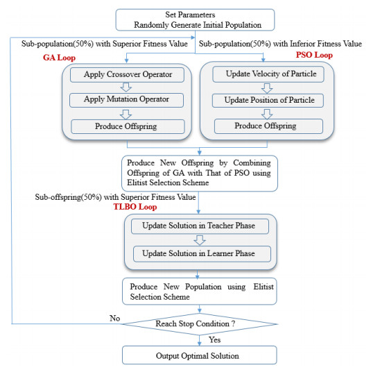
Under addressing global competition, manufacturing companies strive to produce better and cheaper products more quickly. For a complex production system, the design problem is intrinsically a daunting optimization task often involving multiple disciplines, nonlinear mathematical model, and computation-intensive processes during manufacturing process. Here is a reason to develop a high performance algorithm for finding an optimal solution to the engineering design and/or optimization problems. In this paper, a hybrid metaheuristic approach is proposed for solving engineering optimization problems. A genetic algorithm (GA), particle swarm optimization (PSO), and teaching and learning-based optimization (TLBO), called the GA-PSO-TLBO approach, is used and demonstrated for the proposed hybrid metaheuristic approach. Since each approach has its strengths and weaknesses, the GA-PSO-TLBO approach provides an optimal strategy that maintains the strengths as well as mitigates the weaknesses, as needed. The performance of the GA-PSO-TLBO approach is compared with those of conventional approaches such as single metaheuristic approaches (GA, PSO and TLBO) and hybrid metaheuristic approaches (GA-PSO and GA-TLBO) using various types of engineering optimization problems. An additional analysis for reinforcing the performance of the GA-PSO-TLBO approach was also carried out. Experimental results proved that the GA-PSO-TLBO approach outperforms conventional competing approaches and demonstrates high flexibility and efficiency.

| [1] |
M. Gen, Y. Yun, Soft computing approach for reliability optimization: State-of-the-art survey, Rel. Eng. and Sys. Saf., 91 (2006), 1008-1026. https://doi.org/10.1016/j.ress.2005.11.053 doi: 10.1016/j.ress.2005.11.053

|
| [2] |
G. Wang, S. Shan, Review of metamodeling techniques in support of engineering design optimization, Trans. ASME, 129 (2007), 370-380. https://doi.org/10.1115/1.2429697 doi: 10.1115/1.2429697
|
| [3] |
H. M. Amir, T. Hasegawa, Nonlinear mixed-discrete structural optimization, J. Struct. Eng., 115 (1989), 626-646. https://doi.org/10.1061/(ASCE)0733-9445(1989)115:3(626) doi: 10.1061/(ASCE)0733-9445(1989)115:3(626)
|
| [4] |
E. Sandgren, Nonlinear integer and discrete programming in mechanical design optimization, ASME J. Mech. Des., 112 (1990), 223-229. https://doi.org/10.1115/1.2912596 doi: 10.1115/1.2912596
|
| [5] |
J. F. Fu, R. G. Fenton, W. L. Cleghorn, A mixed integer-discrete-continuous programming method and its applications to engineering design optimization, Eng. Opt., 17 (1991), 263-280. https://doi.org/10.1080/03052159108941075 doi: 10.1080/03052159108941075
|
| [6] | W. Kuo, V. R. Prasad, F. Tillman, C. L. Hwang, Optimal reliability design: Fundamentals and applications, Cambridge University Press, 2001. |
| [7] | N. G. Yarushkina, Genetic algorithms for engineering optimization: Theory and practice, in Proceedings of the 2002 IEEE International Conference on Artificial Intelligence System (ICAIS'02), (2002), 357-362. https://doi:10.1109/ICAIS.2002.1048127 |
| [8] |
C. -Y. Lin, P. Hajela, Genetic algorithms in optimization problems with discrete and integer design variables, Eng. Opt., 19 (1992), 309-327. http://doi.org/10.1080/03052159208941234 doi: 10.1080/03052159208941234
|
| [9] |
S. J. Wu, P. T. Chow, Genetic algorithms for nonlinear mixed discrete-integer optimization problems via meta-genetic parameter optimization, Eng. Opt., 24 (1995), 137-159. http://doi.org/10.1080/03052159508941187 doi: 10.1080/03052159508941187
|
| [10] |
T. Yokota, T. Taguchi, M. Gen, A solution method for optimal weight design problem of the gear using genetic algorithms, Comp. Ind. Eng., 35 (1998), 523-526. http://doi.org/10.1016/S0360-8352(98)00149-1 doi: 10.1016/S0360-8352(98)00149-1
|
| [11] |
A. H. Gandomi, X-S. Yang, A. H. Alavi, Cuckoo search algorithm: a metaheuristic approach to solve structural optimization problems, Eng. Comp., 29 (2013), 17-35. http://doi.org/10.1007/s00366-011-0241-y doi: 10.1007/s00366-011-0241-y
|
| [12] | E. S. Maputi, R. Arora, Design optimization of a three-stage transmission using advanced optimization techniques, Int. J. Simul. Multidisci. Des. Opt., 10 (2019). http://doi.org/10.1051/smdo/2019009 |
| [13] |
M. Castelli, L. Vanneschi, Genetic algorithm with variable neighborhood search for the optimal allocation of goods in shop shelves, Oper. Res. Let., 42 (2014), 355-360. http://doi.org/10.1016/j.orl.2014.06.002 doi: 10.1016/j.orl.2014.06.002
|
| [14] |
S. Babaie-Kafaki, R. Ghanbari, N. Mahdavi-Amiri, Hybridizations of genetic algorithms and neighborhood search metaheuristics for fuzzy bus terminal location problems, App. Soft Comp., 46 (2016), 220-229. http://doi.org/10.1016/j.asoc.2016.03.005 doi: 10.1016/j.asoc.2016.03.005
|
| [15] |
O. Dib, M-A. Manier, L. Moalic, A. Caminada. Combining VNS with genetic algorithm to solve the one-to-one routing issue in road networks, Comp. Oper. Res., 78 (2017), 420-430. http://doi.org/10.1016/j.cor.2015.11.010 doi: 10.1016/j.cor.2015.11.010
|
| [16] |
O. Dib, A. Moalic, M-A. Manier, A. Caminada. An advanced GA-VNS combination for multicriteria route planning in public transit networks, Exp. Sys. with Appl., 72 (2017), 67-82. http://doi.org/10.1016/j.eswa.2016.12.009 doi: 10.1016/j.eswa.2016.12.009
|
| [17] |
M. Gen, L. Lin, Y. Yun, H. Inoue, Recent advances in hybrid priority-based genetic algorithms for logistics and SCM network design, Comp. Ind. Eng., 115 (2018), 394-412. http://doi.org/10.1016/j.cie.2018.08.025 doi: 10.1016/j.cie.2018.08.025
|
| [18] |
Y. Yun, A. Chuluunsukh, M. Gen, Sustainable closed-loop supply chain design problem: A hybrid genetic algorithm approach, Mathematics, 8 (2020), 84. http://doi.org/10.3390/math8010084 doi: 10.3390/math8010084
|
| [19] |
I. Sbai, S. Krichen, O. Limam, Two meta-heuristics for solving the capacitated vehicle routing problem: the case of the Tunisian Post Office, Oper. Res., 20 (2020), 2085-2108. http://doi.org/10.1007/s12351-019-00543-8 doi: 10.1007/s12351-019-00543-8
|
| [20] |
J. Wu, M. Fan, Y. Liu, Y. Zhou, N. Yang, M. Yin, A hybrid ant colony algorithm for the winner determination problem, Math. Biosci. Eng., 19 (2022), 3202-3222. http://doi:10.3934/mbe.2022148 doi: 10.3934/mbe.2022148
|
| [21] | Y. Yun, C. U. Moon, Comparison of adaptive genetic algorithm for engineering optimization problems, Int. J. Ind. Eng., 10 (2003), 584-590. |
| [22] | K. Nitisiri, H. Ohwada, M. Gen, Hybrid genetic algorithm with auto-tuning parameters and K-mean clustering strategy for multiple optimization, J. Soc. Plant Eng. Japan, 31 (2019), 58-67. |
| [23] |
Y-T. Kao, E. Zahara, A hybrid genetic algorithm and particle swarm optimization for multimodal functions, Appl. Soft Comp., 8 (2008), 849-857. http://doi.org/10.1016/j.asoc.2007.07.002 doi: 10.1016/j.asoc.2007.07.002
|
| [24] |
X. Huang, Z. Guan, L. Yang, An effective hybrid algorithm for multi-objective flexible job-shop scheduling problem, Adv. Mech. Eng., 10 (2018), 1-14. http://doi.org/10.1177/1687814018801442 doi: 10.1177/1687814018801442
|
| [25] |
M. Güçyetmez, E. Çam, A new hybrid algorithm with genetic-teaching learning optimization (G-TLBO) technique for optimizing of power flow in wind-thermal power systems, Elect. Eng., 98 (2016), 145-157. http://doi.org/10.1007/s00202-015-0357-y doi: 10.1007/s00202-015-0357-y
|
| [26] |
C. J. Shih. Y. C. Yang, Generalized Hopfield network based structural optimization using sequential unconstrained minimization technique with additional penalty strategy, Adv. Eng. Sof., 33 (2002), 721-729. http://doi.org/10.1016/S0965-9978(02)00060-1 doi: 10.1016/S0965-9978(02)00060-1
|
| [27] | Y. Yun, Study on adaptive hybrid genetic algorithm and its applications to engineering design problems, Ph.D. Thesis, Waseda University, Japan, 2005. |
| [28] | D. Kvalie, Optimization of plane elastic grillages, PhD Thesis, Norges Teknisk Naturvitenskapelige Universitet, Norway, 1967. |
| [29] |
T. Ray, P. Saini, Engineering design optimization using a swarm with an intelligent information sharing among individuals, Eng. Opt., 33 (2007), 735-748. http://doi.org/10.1080/03052150108940941 doi: 10.1080/03052150108940941
|
| [30] | A. H. Gandomi, X. S. Yang, Benchmark problems in structural optimization, Chapter 12 in Comp. Opt., Meth. and Alg., (eds. S. Koziel, X-S. Yang) Springer-Verlag, Berlin, (2011), 267-291. http://doi.org/10.1007/978-3-642-20859-1_12 |
| [31] | M. Gen, R. Cheng, Genetic algorithms and engineering optimization, John Wiley & Sons, New York, NY, USA, 2000. |
| [32] | J. Kennedy, R. C. Eberhart, Particle swarm optimization, in Proceedings on IEEE International Conference on Neural Networks, (1995), 1942-1948. http://doi:10.1109/ICNN.1995.488968 |
| [33] | X. Yu, M. Gen, Introduction to evolutionary algorithms, Springer, London, UK, 2010. |
| [34] | R. V. Rao, Teaching learning based optimization algorithm and its engineering applications, Springer, Switzerland, 2016. http://doi.org/10.1007/978-3-319-22732-0_2 |
| [35] | M. Gen, R. Cheng, Genetic algorithms and engineering design, John Wiley and Sons, New York, 1997. |
| [36] | Z. Michalewicz, Genetic algorithms + data structures = evolution program, Spring-Verlag, 1994. |
| [37] |
Y. Marinakis, M. Marinaki, A hybrid genetic - Particle swarm optimization algorithm for the vehicle routing problem, Exp. Syst. Appl., 37 (2010), 1446-1455. http://doi.org/10.1016/j.eswa.2009.06.085 doi: 10.1016/j.eswa.2009.06.085
|
| [38] |
H. Zhai, Y. K. Liu, K. Yang, Modeling two-stage UHL problem with uncertain demands, Appl. Math. Model., 40 (2016), 3029-2048. http://doi.org/10.1016/j.apm.2015.09.086 doi: 10.1016/j.apm.2015.09.086
|
| [39] | M. Gen, A. Chuluunsukh, Y. Yun, Hybridizing teaching-learning based optimization with GA and PSO: Case study of supply chain network model, in the 2021 International Conference on Computational Science and Computational Intelligence (CSCI 2021), Las Vegas, USA, (2021). http://doi:10.1109/CSCI54926.2021.00146 |


Figures(6) / Tables(7)

YoungSu Yun, Mitsuo Gen, Tserengotov Nomin Erdene. Applying GA-PSO-TLBO approach to engineering optimization problems[J]. Mathematical Biosciences and Engineering, 2023, 20(1): 552-571. doi: 10.3934/mbe.2023025


 DownLoad: