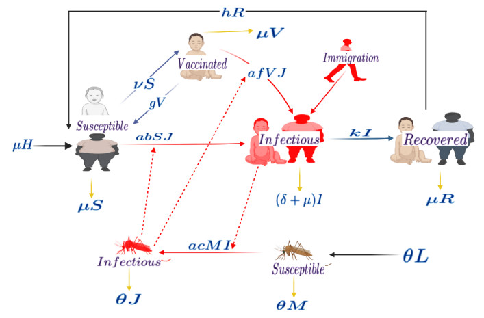
The world is aiming to eliminate malaria by 2030. The introduction of the pilot project on malaria vaccination for children in Kenya, Ghana, and Malawi presents a significant thrust to the elimination efforts. In this work, a susceptible, infectious and recovered (SIR) human-vector interaction mathematical model for malaria was formulated. The model was extended to include a compartment of vaccinated humans and an influx of infected immigrants. Qualitative and quantitative analysis was performed on the model. When there was no influx of infected immigrants, the model had a disease-free equilibrium point that was globally asymptotically stable when a threshold known as the basic reproductive number denoted by $ R_0 $ was less than one. When there was an influx of infected immigrants, the model had endemic equilibrium points only. Parameter sensitivity analysis on $ R_0 $ was performed and results showed that strategies must be implemented to reduce contact between mosquitoes and humans. Results from different vaccine coverage indicated that in the absence of an influx of infected immigrants, it is possible to achieve a malaria-free society when more children get vaccinated and the influx of infected humans is avoided. The analysis of the optimal control model showed that the combined use of vaccination, personal protective equipment, and treatment is the best way to curb malaria incidence, provided the influx of infected humans is completely stopped.
Citation: Pride Duve, Samuel Charles, Justin Munyakazi, Renke Lühken, Peter Witbooi. A mathematical model for malaria disease dynamics with vaccination and infected immigrants[J]. Mathematical Biosciences and Engineering, 2024, 21(1): 1082-1109. doi: 10.3934/mbe.2024045
The world is aiming to eliminate malaria by 2030. The introduction of the pilot project on malaria vaccination for children in Kenya, Ghana, and Malawi presents a significant thrust to the elimination efforts. In this work, a susceptible, infectious and recovered (SIR) human-vector interaction mathematical model for malaria was formulated. The model was extended to include a compartment of vaccinated humans and an influx of infected immigrants. Qualitative and quantitative analysis was performed on the model. When there was no influx of infected immigrants, the model had a disease-free equilibrium point that was globally asymptotically stable when a threshold known as the basic reproductive number denoted by $ R_0 $ was less than one. When there was an influx of infected immigrants, the model had endemic equilibrium points only. Parameter sensitivity analysis on $ R_0 $ was performed and results showed that strategies must be implemented to reduce contact between mosquitoes and humans. Results from different vaccine coverage indicated that in the absence of an influx of infected immigrants, it is possible to achieve a malaria-free society when more children get vaccinated and the influx of infected humans is avoided. The analysis of the optimal control model showed that the combined use of vaccination, personal protective equipment, and treatment is the best way to curb malaria incidence, provided the influx of infected humans is completely stopped.

| [1] | J. Vinetz, What to Know About Malaria, 2022. Available from: https://www.medicalnewstoday.com/articles/150670 |
| [2] | Centers for Disease Control and Prevention, Frequently Asked Questions, 2022. Available from: https://www.cdc.gov/malaria/about/faqs.html |
| [3] | Cleveland Clinic, Malaria Overview, 2022. Available from: https://my.clevelandclinic.org/health/diseases/15014-malaria |
| [4] | World Health Organization, Frequently Asked Questions, 2022. Available from: https://www.who.int/health-topics/malaria |
| [5] |
S. Looareesuwan, J. D. Chulay, C. J. Canfield, D. B. Hutchinson, Malarone (atovaquone and proguanil hydrochloride): A review of its clinical development for treatment of malaria. Malarone Clinical Trials Study Group, Am. J. Trop. Med. Hyg., 60 (1999), 533–541. https://doi.org/10.4269/ajtmh.1999.60.533 doi: 10.4269/ajtmh.1999.60.533

|
| [6] |
S. Dini, S. Zaloumis, P. Cao, R. N. Price, J. Freya, I. Fowkes, et al., Investigating the efficacy of triple artemisinin-based combination therapies for treating Plasmodium falciparum malaria patients using mathematical modeling, Antimicrob. Agents Chemother., 62 (2018). https://doi.org/10.1128/aac.01068-18 doi: 10.1128/aac.01068-18
|
| [7] |
R. Ross, An application of the theory of probabilities to the study of a priori pathometry, Proc. R. Soc. London, 92 (1916), 204–230. https://dx.doi.org/10.1098/rspa.1916.0007 doi: 10.1098/rspa.1916.0007
|
| [8] |
G. Macdonald, Epidemiological basis of malaria control, Bull. W. H. O., 15 (1956), 613. https://dx.doi.org/10.1098/rspa.1916.0007 doi: 10.1098/rspa.1916.0007
|
| [9] |
J. Mohammed-Awel, E. Numfor, R. Zhao, S. Lenhart, A new mathematical model studying imperfect vaccination: Optimal control analysis, J. Math. Anal. Appl., 500 (2021), 125132. https://doi.org/10.1016/j.jmaa.2021.125132 doi: 10.1016/j.jmaa.2021.125132
|
| [10] |
S. Y. Tchoumi, C. W. Chukwu, M. L. Diagne, H. Rwezaura, M. L. Juga, J. M. Tchuenche, Optimal control of a two? Group malaria transmission model with vaccination, Network Model. Anal. Health Inf. Bioinf., 12 (2022), 7. https://doi.org/10.1007/s13721-022-00403-0 doi: 10.1007/s13721-022-00403-0
|
| [11] |
P. Witbooi, G. Abiodun, M. Nsuami, A model of malaria population dynamics with migrants, Math. Biosci. Eng., 18 (2021), 7301–7317. https://dx.doi.org/10.3934/mbe.2021361 doi: 10.3934/mbe.2021361
|
| [12] |
A. Traoré, Analysis of a vector-borne disease model with human and vectors immigration, J. Appl. Math. Comput., 64 (2020), 411–428. https://doi.org/10.1007/s12190-020-01361-4 doi: 10.1007/s12190-020-01361-4
|
| [13] |
D. Heppnerjr, K. Kester, C. Ockenhouse, N. Tornteporth, O. Ofori, J. Lyon, et al., Towards an RTS, S-based, multi-stage, multi-antigen vaccine against falciparum malaria: Progress at the Walter Reed Army Institute of Research, Vaccine, 23 (2005), 2243–2250. http://dx.doi.org/10.1016/j.vaccine.2005.01.142 doi: 10.1016/j.vaccine.2005.01.142
|
| [14] |
M. De la Sen, S. Alonso-Quesada, A. Ibeas, On the stability of an SEIR epidemic model with distributed time-delay and a general class of feedback vaccination rules, Appl. Math. Comput., 270 (2015), 953–976. https://dx.doi.org/10.1016/j.amc.2015.08.099 doi: 10.1016/j.amc.2015.08.099
|
| [15] |
S. Dhiman, Are malaria elimination efforts on right track? An analysis of gains achieved and challenges ahead, Infect. Dis. Poverty, 17 (2019), 1–19. https://doi.org/10.1186/s40249-019-0524-x doi: 10.1186/s40249-019-0524-x
|
| [16] |
European Medicines Agency, First malaria vaccine receives positive scientific opinion, Pharm. J., 2015 (2015). http://dx.doi.org/10.1211/pj.2015.20069061 doi: 10.1211/pj.2015.20069061
|
| [17] | World Health Organization, WHO Malaria Policy Advisory Committee (MPAC) Meeting: Meeting Report, 2022. Available from: https://apps.who.int/iris/handle/10665/312198 |
| [18] |
World Health Organization, Malaria vaccine: WHO position paper–January 2016, Vaccine, 36 (2018), 3576–3577. https://dx.doi.org/10.1016/j.vaccine.2016.10.047 doi: 10.1016/j.vaccine.2016.10.047
|
| [19] |
G. J. Abiodun, P. Witbooi, K. O. Okosun, Modeling and analyzing the impact of temperature and rainfall on mosquito population dynamics over Kwazulu-Natal, South Africa, Int. J. Biomath., 10 (2017), 1750055. https://doi.org/10.1142/S1793524517500553 doi: 10.1142/S1793524517500553
|
| [20] |
K. Okuneye, A. B. Gumel, Analysis of a temperature and rainfall dependent model for malaria transmission dynamics, Math. Biosci., 287 (2017), 72–92. https://doi.org/10.1016/j.mbs.2016.03.013 doi: 10.1016/j.mbs.2016.03.013
|
| [21] |
S. M. Ndiaye, E. M. Parilina, An epidemic model of malaria without and with vaccination. Pt 2. A model of malaria with vaccination, Appl. Math. Comput. Sci. Control Process., 18 (2022), 555–567. https://dx.doi.org/10.21638/11701/spbu10.2022.410 doi: 10.21638/11701/spbu10.2022.410
|
| [22] | World Health Organization, Life Expectancy and Healthy Life Expectancy Data by Country, 2020. Available from: https://apps.who.int/gho/data/node.main.688 |
| [23] |
G. Otieno, J. K. Koske, J. M. Mutiso, Transmission dynamics and optimal control of malaria in Kenya, Discrete Dyn. Nat. Soc., Hindawi Ltd., 2016 (2016), 1–27. https://doi.org/10.1155/2016/8013574 doi: 10.1155/2016/8013574
|
| [24] | M. W. Hirsch, S. Smale, R. L. Devaney, Discrete dynamical systems, in Differential Equations, Dynamical Systems, and an Introduction to Chaos, Academic Press, (2013), 329–-359. https://dx.doi.org/10.1016/b978-0-12-382010-5.00015-4 |
| [25] |
P. van den Driessche, J. Watmough, Reproduction numbers and sub-threshold endemic equilibria for compartmental models of disease transmission, Math. Biosci., 180 (2002), 29–48. https://doi.org/10.1016/S0025-5564(02)00108-6 doi: 10.1016/S0025-5564(02)00108-6
|
| [26] | L. Allen, An Introduction to Mathematical Biology, Prentice Hall, 2007. |
| [27] | J. P. La Salle, The Stability of Dynamical Systems, Society for Industrial and Applied Mathematics, 1976. https://dx.doi.org/10.1137/1.9781611970432 |
| [28] | R. Descartes, La Géométrie, livre premier, édition 1637 publiée dans The geometry of Rene Descartes de David Eugene Smith et Marcia L, 1637. |
| [29] |
C. Castillo-Chavez, B. Song, Dynamical models of tuberculosis and their applications, Math. Biosci. Eng., 1 (2004), 361–404. https://dx.doi.org/10.3934/mbe.2004.1.361 doi: 10.3934/mbe.2004.1.361
|
| [30] |
S. M. Blower, H. Dowlatabadi, Sensitivity and uncertainty analysis of complex models of disease transmission: An HIV model, as an example, Int. Stat. Rev., 62 (1994), 229–243. https://dx.doi.org/10.2307/1403510 doi: 10.2307/1403510
|
| [31] |
S. M. Blower, D. Hartel, H. Dowlatabadi, R. M. Anderson, R.M. May, Sex and HIV: A mathematical model for New York City, Philos. Trans. R. Soc. London Ser. B Biol. Sci., 331 (1991), 171–187. https://dx.doi.org/10.1098/rstb.1991.0006 doi: 10.1098/rstb.1991.0006
|
| [32] |
A. Hoare, D. G. Regan, D. P. Wilson, Sampling and sensitivity analyses tools (SaSAT) for computational modelling, Theor. Biol. Med. Modell., 5 (2008), 1742–4682. https://dx.doi.org/10.1186/1742-4682-5-4 doi: 10.1186/1742-4682-5-4
|
| [33] |
J. Wu, R. Dhingra, M. Gambhir, J. V. Remais, Sensitivity analysis of infectious disease models: Methods, advances and their application, J. R. Soc. Interface, 10, (2013), 1742–5662. https://dx.doi.org/10.1098/rsif.2012.1018 doi: 10.1098/rsif.2012.1018
|
| [34] |
S. Marino, I. B. Hogue, C. J. Ray, D. E. Kirschner, A methodology for performing global uncertainty and sensitivity analysis in systems biology, J. Theor. Biol., 254 (2008), 178–196. https://dx.doi.org/10.1016/j.jtbi.2008.04.011 doi: 10.1016/j.jtbi.2008.04.011
|
| [35] | L. S. Pontryagin, Mathematical Theory of Optimal Processes, CRC press, 1987. |
| [36] | L. S. Pontryagin, V. G. Boltyanskii, R. V. Gamkrelidze, E. F. Mischenko, The Mathematical Theory of Optimal Processes, Cambridge University Press, 1963. |
| [37] |
A. Y. Mukhtar, J. B. Munyakazi, R. Ouifki, Assessing the role of climate factors on malaria transmission dynamics in South Sudan, Math. Biosci., 310 (2019), 13–23. https://doi.org/10.1016/j.mbs.2019.01.002 doi: 10.1016/j.mbs.2019.01.002
|
| [38] |
K. Shah, M. Arfan, A. Ullah, Q. Al-Mdallal, K. J. Ansari, T. Abdeljawad, Computational study on the dynamics of fractional order differential equations with applications, Chaos Solitons Fractals, 157 (2022), 111955. https://dx.doi.org/10.1016/j.chaos.2022.111955 doi: 10.1016/j.chaos.2022.111955
|
| [39] |
K. Hattaf, A new class of generalized fractal and fractal-fractional derivatives with non-singular kernels, Fractal Fractional, 5 (2023), 395. https://dx.doi.org/10.3390/fractalfract7050395 doi: 10.3390/fractalfract7050395
|
| [40] |
M. Semlali, K. Hattaf, E. K. Mohamed, Modeling and analysis of the dynamics of COVID-19 transmission in presence of immigration and vaccination, Commun. Math. Biol. Neurosci., 2002 (2022). https://dx.doi.org/10.28919/cmbn/7270 doi: 10.28919/cmbn/7270
|
| [41] |
N. Sene, SIR epidemic model with Mittag-Leffler fractional derivative, Chaos Solitons Fractals, 137 (2020), 109833. https://dx.doi.org/10.1016/j.chaos.2020.109833 doi: 10.1016/j.chaos.2020.109833
|
| [42] |
P. J. Witbooi, S. M. Vyambwera, G. J. van Schalkwyk, G. E. Muller, Stability and control in a stochastic model of malaria population dynamics, Adv. Contin. Discrete Models, 1 (2023), 45. https://dx.doi.org/10.1186/s13662-023-03791-3 doi: 10.1186/s13662-023-03791-3
|


Figures(10) / Tables(2)

Pride Duve, Samuel Charles, Justin Munyakazi, Renke Lühken, Peter Witbooi. A mathematical model for malaria disease dynamics with vaccination and infected immigrants[J]. Mathematical Biosciences and Engineering, 2024, 21(1): 1082-1109. doi: 10.3934/mbe.2024045


 DownLoad: