SE-TCN network for continuous estimation of upper limb joint angles

Xiaoguang Liu; Jiawei Wang; Tie Liang; Cunguang Lou; Hongrui Wang; Xiuling Liu; Xiaoguang Liu; Jiawei Wang; Tie Liang; Cunguang Lou; Hongrui Wang; Xiuling Liu

doi:10.3934/mbe.2023152

Mathematical Biosciences and Engineering

2023, Volume 20, Issue 2: 3237-3260. doi: 10.3934/mbe.2023152

Previous Article Next Article

Research article

SE-TCN network for continuous estimation of upper limb joint angles

1.
College of Electronic and Information Engineering, Hebei University, Baoding, Hebei, China
2.
Key Laboratory of Digital Medical Engineering of Hebei Province, Hebei University, Baoding, Hebei, China

Academic Editor: Vladimir Mityushev

Received: 23 August 2022 Revised: 22 November 2022 Accepted: 23 November 2022 Published: 02 December 2022

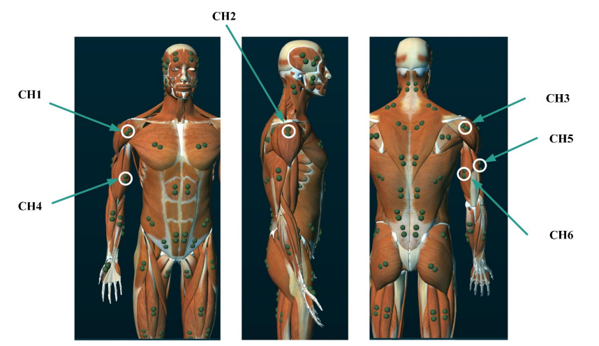
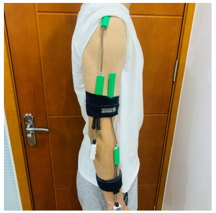
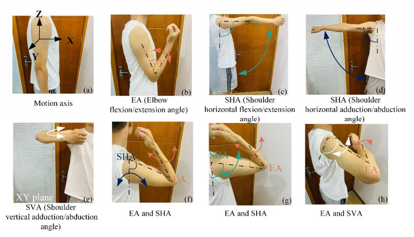
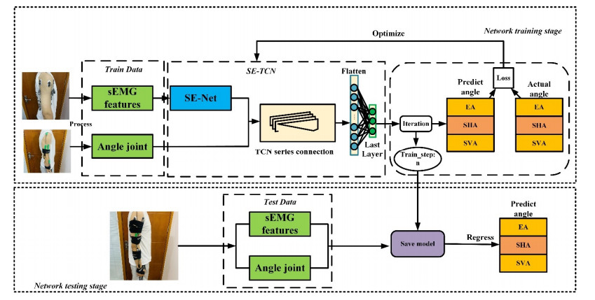
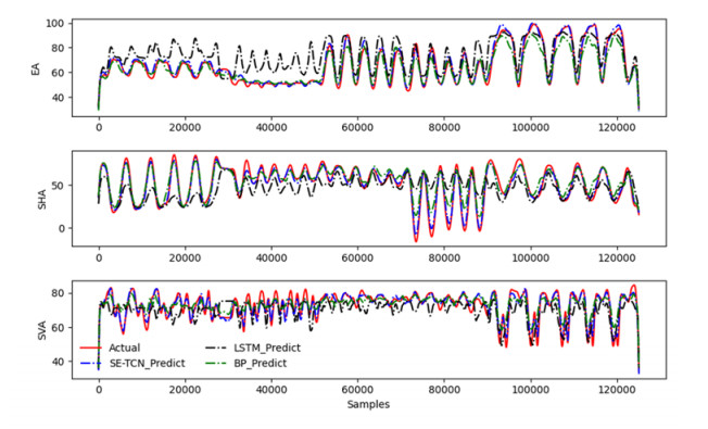
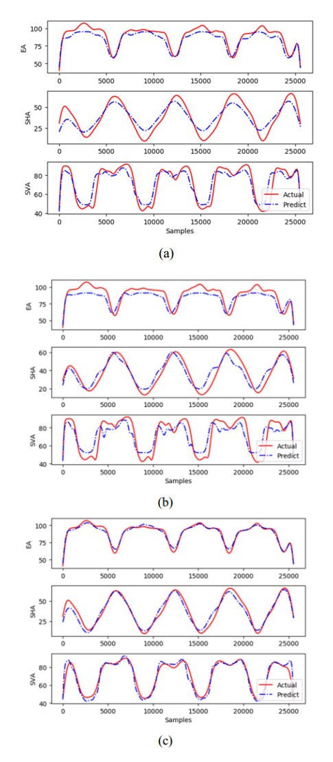
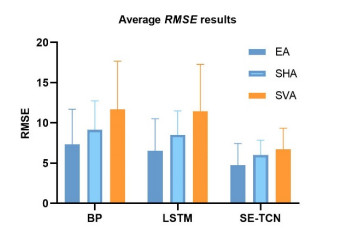
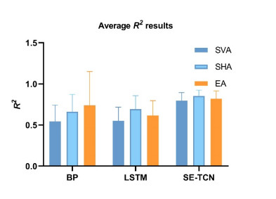
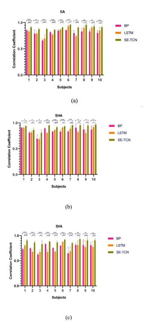
The maturity of human-computer interaction technology has made it possible to use surface electromyographic signals (sEMG) to control exoskeleton robots and intelligent prostheses. However, the available upper limb rehabilitation robots controlled by sEMG have the shortcoming of inflexible joints. This paper proposes a method based on a temporal convolutional network (TCN) to predict upper limb joint angles by sEMG. The raw TCN depth was expanded to extract the temporal features and save the original information. The timing sequence characteristics of the muscle blocks that dominate the upper limb movement are not apparent, leading to low accuracy of the joint angle estimation. Therefore, this study squeeze-and-excitation networks (SE-Net) to improve the network model of the TCN. Finally, seven movements of the human upper limb were selected for ten human subjects, recording elbow angle (EA), shoulder vertical angle (SVA), and shoulder horizontal angle (SHA) values during their movements. The designed experiment compared the proposed SE-TCN model with the backpropagation (BP) and long short-term memory (LSTM) networks. The proposed SE-TCN systematically outperformed the BP network and LSTM model by the mean RMSE values: by 25.0 and 36.8% for EA, by 38.6 and 43.6% for SHA, and by 45.6 and 49.5% for SVA, respectively. Consequently, its R² values exceeded those of BP and LSTM by 13.6 and 39.20% for EA, 19.01 and 31.72% for SHA, and 29.22 and 31.89% for SVA, respectively. This indicates that the proposed SE-TCN model has good accuracy and can be used to estimate the angles of upper limb rehabilitation robots in the future.
- continuous angle estimation,
- human-computer interaction,
- sEMG,
- SE-TCN network
Citation: Xiaoguang Liu, Jiawei Wang, Tie Liang, Cunguang Lou, Hongrui Wang, Xiuling Liu. SE-TCN network for continuous estimation of upper limb joint angles[J]. Mathematical Biosciences and Engineering, 2023, 20(2): 3237-3260. doi: 10.3934/mbe.2023152

Related Papers:

Abstract

The maturity of human-computer interaction technology has made it possible to use surface electromyographic signals (sEMG) to control exoskeleton robots and intelligent prostheses. However, the available upper limb rehabilitation robots controlled by sEMG have the shortcoming of inflexible joints. This paper proposes a method based on a temporal convolutional network (TCN) to predict upper limb joint angles by sEMG. The raw TCN depth was expanded to extract the temporal features and save the original information. The timing sequence characteristics of the muscle blocks that dominate the upper limb movement are not apparent, leading to low accuracy of the joint angle estimation. Therefore, this study squeeze-and-excitation networks (SE-Net) to improve the network model of the TCN. Finally, seven movements of the human upper limb were selected for ten human subjects, recording elbow angle (EA), shoulder vertical angle (SVA), and shoulder horizontal angle (SHA) values during their movements. The designed experiment compared the proposed SE-TCN model with the backpropagation (BP) and long short-term memory (LSTM) networks. The proposed SE-TCN systematically outperformed the BP network and LSTM model by the mean RMSE values: by 25.0 and 36.8% for EA, by 38.6 and 43.6% for SHA, and by 45.6 and 49.5% for SVA, respectively. Consequently, its R² values exceeded those of BP and LSTM by 13.6 and 39.20% for EA, 19.01 and 31.72% for SHA, and 29.22 and 31.89% for SVA, respectively. This indicates that the proposed SE-TCN model has good accuracy and can be used to estimate the angles of upper limb rehabilitation robots in the future.

References

[1]	L. Vodovnik, C. Long, J. B. Reswick, A. Lippay, D. Starbuck, Myo-electric control of paralyzed muscles, IEEE Trans. Biomed. Eng., BME-12 (1965), 169–172. https://doi.org/10.1109/tbme.1965.4502374 doi: 10.1109/tbme.1965.4502374
[2]	W. Geng, Y. Du, W. Jin, W. Wei, Y. Hu, J. Li, Gesture recognition by instantaneous surface EMG images, Sci. Rep., 6 (2016), 36571. https://doi.org/10.1038/srep36571 doi: 10.1038/srep36571
[3]	P. Tsarouchi, S. Makris, G. Chryssolouris, Human-robot interaction review and challenges on task planning and programming, Int. J. Comput. Integr. Manuf., 29 (2016), 916–931. https://doi.org/10.1080/0951192X.2015.1130251 doi: 10.1080/0951192X.2015.1130251
[4]	C. Yang, C. Zeng, P. Liang, Z. Li, R. Li, C. Su, Interface design of a physical human–robot interaction system for human impedance adaptive skill transfer, IEEE Trans. Autom. Sci. Eng., 15 (2017), 329–340.
[5]	M. Bowman, J. Zhang, X. Zhang, An intent-based task-aware shared control framework for intuitive hands free telemanipulation, preprint, arXiv: 2003.03677. https://doi.org/10.48550/arXiv.2003.03677
[6]	S. Li, H. Wang, M. U. Rafique, A novel recurrent neural network for manipulator control with improved noise tolerance, IEEE Trans. Neural Networks Learn. Syst., 29 (2017), 1908–1918. https://doi.org/10.1109/TNNLS.2017.2672989 doi: 10.1109/TNNLS.2017.2672989
[7]	D. Zhang, Z. Wu, J. Chen, R. Zhu, A. Munawar, B. Xiao, et al., Human-robot shared control for surgical robot based on context-aware sim-to-real adaptation, preprint, arXiv: 2204.11116. https://doi.org/10.48550/arXiv.2204.11116
[8]	R. Bertani, C. Melegari, M. C. De Cola, A. Bramanti, P. Bramanti, R. S. Calabrò, Effects of robot-assisted upper limb rehabilitation in stroke patients: a systematic review with meta-analysis, Neurol. Sci., 38 (2017), 1561–1569. https://doi.org/10.1007/s10072-017-2995-5 doi: 10.1007/s10072-017-2995-5
[9]	P. Maciejasz, J. Eschweiler, K. Gerlach-Hahn, A. Jansen-Troy, S. Leonhardt, A survey on robotic devices for upper limb rehabilitation, J. NeuroEng. Rehabil., 11 (2014), 1–29. https://doi.org/10.1186/1743-0003-11-3 doi: 10.1186/1743-0003-11-3
[10]	A. J. Young, L. H. Smith, E. J. Rouse, L. J. Hargrove, Classification of simultaneous movements using surface EMG pattern recognition, IEEE Trans. Biomed. Eng., 60 (2012), 1250–1258. https://doi.org/10.1109/TBME.2012.2232293 doi: 10.1109/TBME.2012.2232293
[11]	X. Wu, W. Hou, X. Zheng, H. Wang, M. Zha, Relationship between surface EMG and angle of elbow joint, Space Med. Med. Eng., 6 (2006).
[12]	N. K. Karnam, A. C. Turlapaty, S. R. Dubey, B. Gokaraju, Classification of sEMG signals of hand gestures based on energy features, Biomed. Signal Process. Control, 70 (2021), 102948. https://doi.org/10.1016/j.bspc.2021.102948 doi: 10.1016/j.bspc.2021.102948
[13]	B. Hudgins, P. Parker, R. N. Scott, A new strategy for multifunction myoelectric control, IEEE Trans. Biomed. Eng., 40 (1993), 82–94. https://doi.org/10.1109/10.204774 doi: 10.1109/10.204774
[14]	J. Rafiee, M. A. Rafiee, F. Yavari, M. P. Schoen, Feature extraction of forearm EMG signals for prosthetics, Expert Syst. Appl., 38 (2011), 4058–4067. https://doi.org/10.1016/j.eswa.2010.09.068 doi: 10.1016/j.eswa.2010.09.068
[15]	J. Wang, Q. Hao, X. Xi, J. Cao, A. Xue, H. Wang, Estimation of continuous joint angles of upper limb based on sEMG by using GA-Elman neural network, Math. Probl. Eng., 2020 (2020).
[16]	G. Tang, J. Sheng, D. Wang, S. Men, Continuous estimation of human upper limb joint angles by using PSO-LSTM model, IEEE Access, 9 (2020), 17986–17997. https://doi.org/10.1109/ACCESS.2020.3047828 doi: 10.1109/ACCESS.2020.3047828
[17]	A. Phinyomark, P. Phukpattaranont, C. Limsakul, Feature reduction and selection for EMG signal classification, Expert Syst. Appl., 39 (2012), 7420–7431. https://doi.org/10.1016/j.eswa.2012.01.102 doi: 10.1016/j.eswa.2012.01.102
[18]	A. Phinyomark, R. N. Khushaba, E. Scheme, Feature extraction and selection for myoelectric control based on wearable EMG sensors, Sensors, 18 (2018), 1615. https://doi.org/10.3390/s18051615 doi: 10.3390/s18051615
[19]	S. Bai, J. Z. Kolter, V. Koltun, An empirical evaluation of generic convolutional and recurrent networks for sequence modeling, preprint, arXiv: 1803.01271. https://doi.org/10.48550/arXiv.1803.01271
[20]	P. Liu, X. Qiu, X. Huang, Recurrent neural network for text classification with multi-task learning, preprint, arXiv: 1605.05101. https://doi.org/10.48550/arXiv.1605.05101
[21]	S. Hochreiter, J. Schmidhuber, Long short-term memory, Neural Comput., 9 (1997), 1735–1780. https://doi.org/10.1162/neco.1997.9.8.1735 doi: 10.1162/neco.1997.9.8.1735
[22]	C. Lea, M. D. Flynn, R. Vidal, A. Reiter, G. D. Hager, Temporal convolutional networks for action segmentation and detection, in 2017 IEEE Conference on Computer Vision and Pattern Recognition (CVPR), (2017), 156–165. https://doi.org/10.1109/CVPR.2017.113
[23]	J. Zhu, L. Su, Y. Li, Wind power forecasting based on new hybrid model with TCN residual modification, Energy AI, 10 (2022), 100199. https://doi.org/10.1016/j.egyai.2022.100199 doi: 10.1016/j.egyai.2022.100199
[24]	X. Guo, Q. Wang, J. Zheng, An intelligent computer-aided diagnosis approach for atrial fibrillation detection based on multi-scale convolution kernel and Squeeze-and-Excitation network, Biomed. Signal Process. Control, 68 (2021), 102778. https://doi.org/10.1016/j.bspc.2021.102778 doi: 10.1016/j.bspc.2021.102778
[25]	J. Hu, L. Shen, G. Sun, Squeeze-and-excitation networks, in 2018 IEEE/CVF Conference on Computer Vision and Pattern Recognition, (2018), 7132–7141. https://doi.org/10.1109/CVPR.2018.00745
[26]	Y. M. Aung, A. Al-Jumaily, Estimation of upper limb joint angle using surface EMG signal, Int. J. Adv. Rob. Syst., 10 (2013), 369. https://doi.org/10.5772/56717 doi: 10.5772/56717
[27]	M. Abadi, P. Barham, J. Chen, Z. Chen, A. Davis, J. Dean, et al., {TensorFlow}: a system for {Large-Scale} machine learning, in 12th USENIX symposium on operating systems design and implementation (OSDI 16), (2016), 265–283.

Reader Comments

Your name:*

Email:*
© 2023 the Author(s), licensee AIMS Press. This is an open access article distributed under the terms of the Creative Commons Attribution License (http://creativecommons.org/licenses/by/4.0)