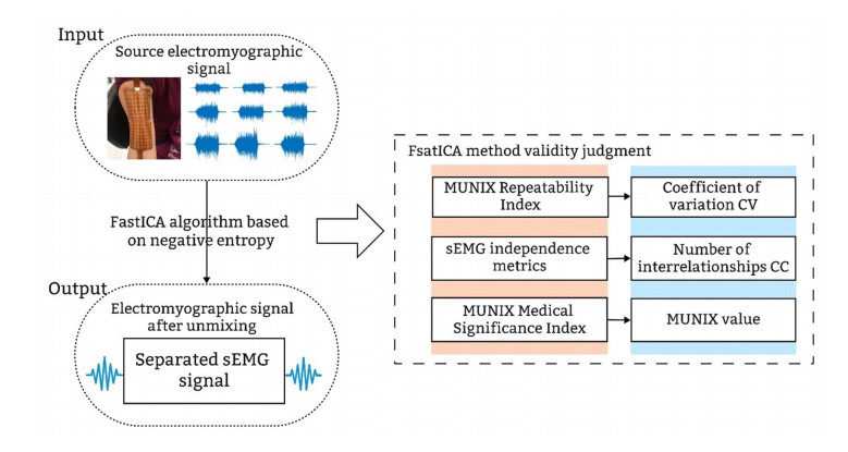
To enhance the reproducibility of motor unit number index (MUNIX) for evaluating neurological disease progression, this paper proposes a negative entropy-based fast independent component analysis (FastICA) demixing method to assess MUNIX reproducibility in the presence of inter-channel mixing of electromyography (EMG) signals acquired by high-density electrodes. First, composite surface EMG (sEMG) signals were obtained using high-density surface electrodes. Second, the FastICA algorithm based on negative entropy was employed to determine the orthogonal projection matrix that minimizes the negative entropy of the projected signal and effectively separates mixed sEMG signals. Finally, the proposed experimental approach was validated by introducing an interrelationship criterion to quantify independence between adjacent channel EMG signals, measuring MUNIX repeatability using coefficient of variation (CV), and determining motor unit number and size through MUNIX. Results analysis shows that the inclusion of the full (128) channel sEMG information leads to a reduction in CV value by $1.5 \pm 0.1$ and a linear decline in CV value with an increase in the number of channels. The correlation between adjacent channels in participants decreases by $0.12 \pm 0.05$ as the number of channels gradually increases. The results demonstrate a significant reduction in the number of interrelationships between sEMG signals following negative entropy-based FastICA processing, compared to the mixed sEMG signals. Moreover, this decrease in interrelationships becomes more pronounced with an increasing number of channels. Additionally, the CV of MUNIX gradually decreases with an increase in the number of channels, thereby optimizing the issue of abnormal MUNIX repeatability patterns and further enhancing the reproducibility of MUNIX based on high-density surface EMG signals.
Citation: Suqi Xue, Farong Gao, Xudong Wu, Qun Xu, Xuecheng Weng, Qizhong Zhang. MUNIX repeatability evaluation method based on FastICA demixing[J]. Mathematical Biosciences and Engineering, 2023, 20(9): 16362-16382. doi: 10.3934/mbe.2023730
To enhance the reproducibility of motor unit number index (MUNIX) for evaluating neurological disease progression, this paper proposes a negative entropy-based fast independent component analysis (FastICA) demixing method to assess MUNIX reproducibility in the presence of inter-channel mixing of electromyography (EMG) signals acquired by high-density electrodes. First, composite surface EMG (sEMG) signals were obtained using high-density surface electrodes. Second, the FastICA algorithm based on negative entropy was employed to determine the orthogonal projection matrix that minimizes the negative entropy of the projected signal and effectively separates mixed sEMG signals. Finally, the proposed experimental approach was validated by introducing an interrelationship criterion to quantify independence between adjacent channel EMG signals, measuring MUNIX repeatability using coefficient of variation (CV), and determining motor unit number and size through MUNIX. Results analysis shows that the inclusion of the full (128) channel sEMG information leads to a reduction in CV value by $1.5 \pm 0.1$ and a linear decline in CV value with an increase in the number of channels. The correlation between adjacent channels in participants decreases by $0.12 \pm 0.05$ as the number of channels gradually increases. The results demonstrate a significant reduction in the number of interrelationships between sEMG signals following negative entropy-based FastICA processing, compared to the mixed sEMG signals. Moreover, this decrease in interrelationships becomes more pronounced with an increasing number of channels. Additionally, the CV of MUNIX gradually decreases with an increase in the number of channels, thereby optimizing the issue of abnormal MUNIX repeatability patterns and further enhancing the reproducibility of MUNIX based on high-density surface EMG signals.

| [1] |
A. A. Lari, A. A. Ghavanini, H. R. Bokaee, A review of electrophysiological studies of lower motor neuron involvement in amyotrophic lateral sclerosis, Neurol. Sci., 40 (2019), 1125–1136. https://doi.org/10.1007/s10072-019-03832-4 doi: 10.1007/s10072-019-03832-4

|
| [2] |
J. Nijssen, L. H. Comley, E. Hedlund, Motor neuron vulnerability and resistance in amyotrophic lateral sclerosis, Acta Neuropathol., 133 (2017), 863–885. https://doi.org/10.1007/s00401-017-1708-8 doi: 10.1007/s00401-017-1708-8
|
| [3] |
S. D. Nandedkar, D. S. Nandedkar, P. E. Barkhaus, E. V. Stalberg, Motor unit number index (MUNIX), IEEE Trans. Biomed. Eng., 51 (2004), 2209–2211. https://doi.org/10.1109/TBME.2004.834281 doi: 10.1109/TBME.2004.834281
|
| [4] |
S. D. Nandedkar, P. E. Barkhaus, E. V. StÅlberg, Motor unit number index (MUNIX): principle, method, and findings in healthy subjects and in patients with motor neuron disease, Muscle Nerve, 42 (2010), 798–807. https://doi.org/10.1002/mus.21824 doi: 10.1002/mus.21824
|
| [5] |
Q. Xu, S. Xue, F. Gao, Q. Wu, Q. Zhang, Evaluation method of motor unit number index based on optimal muscle strength combination, Math. Biosci. Eng., 20 (2023), 3854–3872. https://doi.org/10.3934/mbe.2023181 doi: 10.3934/mbe.2023181
|
| [6] |
W. A. Boekestein, H. J. Schelhaas, M. J. A. M. van Putten, D. F. Stegeman, M. J. Zwarts, J. P. van Dijk, Motor unit number index (MUNIX) versus motor unit number estimation (MUNE): a direct comparison in a longitudinal study of ALS patients, Clin. Neurophysiol., 123 (2012), 1644–1649. https://doi.org/10.1016/j.clinph.2012.01.004 doi: 10.1016/j.clinph.2012.01.004
|
| [7] |
C. Neuwirth, P. E. Barkhaus, C. Burkhardt, J. Castro, D. Czell, M. de Carvalho, et al., Tracking motor neuron loss in a set of six muscles in amyotrophic lateral sclerosis using the motor unit number index (MUNIX): a 15-month longitudinal multicentre trial, J. Neurol. Neurosurg. Psychiatry, 86 (2015), 1172–1179. https://doi.org/10.1136/jnnp-2015-310509 doi: 10.1136/jnnp-2015-310509
|
| [8] |
J. Furtula, B. Johnsen, P. B. Christensen, K. Pugdahl, C. Bisgaard, M. K. Christensen, et al., MUNIX and incremental stimulation MUNE in ALS patients and control subjects, Clin. Neurophysiol., 124 (2013), 610–618. https://doi.org/10.1016/j.clinph.2012.08.023 doi: 10.1016/j.clinph.2012.08.023
|
| [9] |
S. D. Nandedkar, P. E. Barkhaus, E. V. Stålberg, Reproducibility of MUNIX in patients with amyotrophic lateral sclerosis, Muscle Nerve, 44 (2011), 919–922. https://doi.org/10.1002/mus.22204 doi: 10.1002/mus.22204
|
| [10] |
C. Neuwirth, S. Nandedkar, E. Stålberg, P. E. Barkhaus, M. de Carvalho, J. Furtula, et al., Motor unit number index (MUNIX): a novel neurophysiological marker for neuromuscular disorders; test-retest reliability in healthy volunteers, Clin. Neurophysiol., 122 (2011), 1867–1872. https://doi.org/10.1016/j.clinph.2011.02.017 doi: 10.1016/j.clinph.2011.02.017
|
| [11] |
N. Dias, X. Li, C. Zhang, Y. Zhang, Innervation asymmetry of the external anal sphincter in aging characterized from high-density intra-rectal surface EMG recordings, Neurourol. Urodyn., 37 (2018), 2544–2550. https://doi.org/10.1002/nau.23809 doi: 10.1002/nau.23809
|
| [12] |
R. Günther, C. Neuwirth, J. C. Koch, P. Lingor, N. Braun, R. Untucht, et al., Motor unit number index (MUNIX) of hand muscles is a disease biomarker for adult spinal muscular atrophy, Clin. Neurophysiol., 130 (2019), 315–319. https://doi.org/10.1016/j.clinph.2018.11.009 doi: 10.1016/j.clinph.2018.11.009
|
| [13] |
C. Neuwirth, C. Burkhardt, J. Alix, J. Castro, M. de Carvalho, M. Gawel, et al., Quality control of motor unit number index (MUNIX) measurements in 6 muscles in a single-subject "round-robin" setup, PLoS One, 11 (2016), e0153948. https://doi.org/10.1371/journal.pone.0153948 doi: 10.1371/journal.pone.0153948
|
| [14] |
S. W. Ahn, S. H. Kim, J. E. Kim, S. M. Kim, S. H. Kim, K. S. Park, et al., Reproducibility of the motor unit number index (MUNIX) in normal controls and amyotrophic lateral sclerosis patients, Muscle Nerve, 42 (2010), 808–813. https://doi.org/10.1002/mus.21765 doi: 10.1002/mus.21765
|
| [15] |
C. Neuwirth, N. Braun, K. G. Claeys, R. Bucelli, C. Fournier, M. Bromberg, et al., Implementing motor unit number index (MUNIX) in a large clinical trial: Real world experience from 27 centres, Clin. Neurophysiol., 129 (2018), 1756–1762. https://doi.org/10.1016/j.clinph.2018.04.614 doi: 10.1016/j.clinph.2018.04.614
|
| [16] |
D. Fathi, B. Mohammadi, R. Dengler, S. Böselt, S. Petri, K. Kollewe, Lower motor neuron involvement in ALS assessed by motor unit number index (MUNIX): long-term changes and reproducibility, Clin. Neurophysiol., 127 (2016), 1984–1988. https://doi.org/10.1016/j.clinph.2015.12.023 doi: 10.1016/j.clinph.2015.12.023
|
| [17] |
C. Neuwirth, S. Nandedkar, E. StåLberg, M. Weber, Motor unit number index (MUNIX): a novel neurophysiological technique to follow disease progression in amyotrophic lateral sclerosis, Muscle Nerve, 42 (2010), 379–384. https://doi.org/10.1002/mus.21707 doi: 10.1002/mus.21707
|
| [18] |
F. Fatehi, E. Delmont, A. M. Grapperon, E. Salort-Campana, A. Sévy, A. Verschueren, et al., Motor unit number index (MUNIX) in patients with anti-MAG neuropathy, Clin. Neurophysiol., 128 (2017), 1264–1269. https://doi.org/10.1016/j.clinph.2017.04.022 doi: 10.1016/j.clinph.2017.04.022
|
| [19] |
F. Fatehi, A. M. Grapperon, D. Fathi, E. Delmont, S. Attarian, The utility of motor unit number index: a systematic review, Neurophysiol. Clin., 48 (2018), 251–259. https://doi.org/10.1016/j.neucli.2018.09.001 doi: 10.1016/j.neucli.2018.09.001
|
| [20] |
E. Issoglio, P. Smith, J. Voss, On the estimation of entropy in the FastICA algorithm, J. Multivar. Anal., 181 (2021), 104689. https://doi.org/10.1016/j.jmva.2020.104689 doi: 10.1016/j.jmva.2020.104689
|
| [21] |
F. Gao, Y. Cao, C. Zhang, Y. Zhang, A preliminary study of effects of channel number and location on the repeatability of motor unit number index (MUNIX), Front. Neurol., 11 (2020), 191. https://doi.org/10.3389/fneur.2020.00191 doi: 10.3389/fneur.2020.00191
|
| [22] |
Y. Peng, J. He, B. Yao, S. Li, P. Zhou, Y. Zhang, Motor unit number estimation based on high-density surface electromyography decomposition, Clin. Neurophysiol., 127 (2016), 3059–3065. https://doi.org/10.1016/j.clinph.2016.06.014 doi: 10.1016/j.clinph.2016.06.014
|
| [23] |
B. Cao, X. Gu, L. Zhang, Y. Hou, Y. Chen, Q. Wei, et al., Reference values for the motor unit number index and the motor unit size index in five muscles, Muscle Nerve, 61 (2020), 657–661. https://doi.org/10.1002/mus.26837 doi: 10.1002/mus.26837
|
| [24] | Q. Li, J. Yang, Research on the surface electromyography signal decomposition based on multi-channel signal fusion analysis, J. Biomed. Eng., 29 (2012), 948–953. |
| [25] |
A. Hyvarinen, Fast and robust fixed-point algorithms for independent component analysis, IEEE Trans. Neural Networks, 10 (1999), 626–634. https://doi.org/10.1109/72.761722 doi: 10.1109/72.761722
|
| [26] |
Z. Liu, D. Yang, Y. Wang, M. Lu, R. Li, EGNN: Graph structure learning based on evolutionary computation helps more in graph neural networks, Appl. Soft Comput., 135 (2023), 110040. https://doi.org/10.1016/j.asoc.2023.110040 doi: 10.1016/j.asoc.2023.110040
|
| [27] |
M. L. Escorcio-Bezerra, A. Abrahao, D. Santos-Neto, N. I. de Oliveira Braga, A. S. B. Oliveira, G. M. Manzano, et al., Why averaging multiple MUNIX measures in the longitudinal assessment of patients with ALS? Clin. Neurophysiol., 128 (2017), 2392–2396. https://doi.org/10.1016/j.clinph.2017.09.104 doi: 10.1016/j.clinph.2017.09.104
|
| [28] |
C. Dai, X. Hu, Independent component analysis based algorithms for high-density electromyogram decomposition: experimental evaluation of upper extremity muscles, Comput. Biol. Med., 108 (2019), 42–48. https://doi.org/10.1016/j.compbiomed.2019.03.009 doi: 10.1016/j.compbiomed.2019.03.009
|
| [29] |
J. Thomas, Y. Deville, S. Hosseini, Differential fast fixed-point algorithms for underdetermined instantaneous and convolutive partial blind source separation, IEEE Trans. Signal Process., 55 (2007), 3717–3729. https://doi.org/10.1109/TSP.2007.894243 doi: 10.1109/TSP.2007.894243
|
| [30] |
M. Chen, X. Zhang, Z. Lu, X. Li, P. Zhou, Two-source validation of progressive FastICA peel-off for automatic surface EMG decomposition in human first dorsal interosseous muscle, Int. J. Neural Syst., 28 (2018), 1850019. https://doi.org/10.1142/S0129065718500193 doi: 10.1142/S0129065718500193
|
| [31] |
M. Chen, X. Zhang, P. Zhou, A novel validation approach for high density surface EMG decomposition in motor neuron disease, IEEE Trans. Neural Syst. Rehabil. Eng., 26 (2018), 1161–1168. https://doi.org/10.1109/TNSRE.2018.2836859 doi: 10.1109/TNSRE.2018.2836859
|
| [32] |
M. Liu, J. Yang, E. Fan, J. Qiu, W. Zheng, Leak location procedure based on the complex-valued FastICA blind deconvolution algorithm for water-filled branch pipe, Water Supply, 22 (2022), 2560–2572. https://doi.org/10.2166/ws.2021.450 doi: 10.2166/ws.2021.450
|
| [33] |
M. Chen, P. Zhou, Automatic decomposition of pediatric high density surface EMG: a pilot study, Med. Novel Technol. Devices, 12 (2021), 100094. https://doi.org/10.1016/j.medntd.2021.100094 doi: 10.1016/j.medntd.2021.100094
|
| [34] |
M. Drey, C. Grösch, C. Neuwirth, J. M. Bauer, C. C. Sieber, The motor unit number index (MUNIX) in sarcopenic patients, Exp. Gerontol., 48 (2013), 381–384. https://doi.org/10.1016/j.exger.2013.01.011 doi: 10.1016/j.exger.2013.01.011
|
| [35] |
W. Qi, S. E. Ovur, Z. Li, A. Marzullo, R. Song, Multi-sensor guided and gesture recognition for a teleoperated robot using a recurrent neural network, IEEE Rob. Autom. Lett., 6 (2021), 6039–6045. https://doi.org/10.1109/LRA.2021.3089999 doi: 10.1109/LRA.2021.3089999
|
| [36] |
W. Qi, H. Su, A cybertwin based multimodal network for ECG patterns monitoring using deep learning, IEEE Trans. Ind. Inf., 18 (2022), 6663–6670. https://doi.org/10.1109/TⅡ.2022.3159583 doi: 10.1109/TⅡ.2022.3159583
|
| [37] |
C. Tian, Z. Xu, L. Wang, Y. Liu, Arc fault detection using artificial intelligence: challenges and benefits, Math. Biosci. Eng., 20 (2023), 12404–12432. https://doi.org/10.3934/mbe.2023552 doi: 10.3934/mbe.2023552
|
| [38] |
Y. Shi, L. Li, J. Yang, Y. Wang, S. Hao, Center-based transfer feature learning with classifier adaptation for surface defect recognition, Mech. Syst. Signal Process., 188 (2023), 110001. https://doi.org/10.1016/j.ymssp.2022.110001 doi: 10.1016/j.ymssp.2022.110001
|
| [39] |
Y. Wang, Z. Liu, J. Xu, W. Yan, Heterogeneous network representation learning approach for ethereum identity identification, IEEE Trans. Comput. Social Syst., 10 (2023), 890–899. https://doi.org/10.1109/TCSS.2022.3164719 doi: 10.1109/TCSS.2022.3164719
|
| [40] |
M. Gawel, M. Kuzma-Kozakiewicz, Does the MUNIX method reflect clinical dysfunction in amyotrophic lateral sclerosis: a practical experience, Medicine, 95 (2016), e3647. https://doi.org/10.1097/MD.0000000000003647 doi: 10.1097/MD.0000000000003647
|
| [41] |
S. Li, J. Liu, M. Bhadane, P. Zhou, W. Z. Rymer, Activation deficit correlates with weakness in chronic stroke: evidence from evoked and voluntary EMG recordings, Clin. Neurophysiol., 125 (2014), 2413–2417. https://doi.org/10.1016/j.clinph.2014.03.019 doi: 10.1016/j.clinph.2014.03.019
|
| [42] |
Y. Peng, Y. C. Zhang, Improving the repeatability of motor unit number index (MUNIX) by introducing additional epochs at low contraction levels, Clin. Neurophysiol., 128 (2017), 1158–1165. https://doi.org/10.1016/j.clinph.2017.03.044 doi: 10.1016/j.clinph.2017.03.044
|
| [43] |
C. W. Chin, A short and elementary proof of the central limit theorem by individual swapping, Am. Math. Mon., 129 (2022), 374–380. https://doi.org/10.1080/00029890.2022.2027711 doi: 10.1080/00029890.2022.2027711
|
| [44] |
J. Miettinen, K. Nordhausen, H. Oja, S. Taskinen, Deflation-based FastICA with adaptive choices of nonlinearities, IEEE Trans. Signal Process., 62 (2014), 5716–5724. https://doi.org/10.1109/TSP.2014.2356442 doi: 10.1109/TSP.2014.2356442
|
| [45] |
J. P. van Dijk, J. H. Blok, B. G. Lapatki, I. N. van Schaik, M. J. Zwarts, D. F. Stegeman, Motor unit number estimation using high-density surface electromyography, Clin. Neurophysiol., 119 (2008), 33–42. https://doi.org/10.1016/j.clinph.2007.09.133 doi: 10.1016/j.clinph.2007.09.133
|
| [46] |
X. Li, Y. C. Wang, N. L. Suresh, W. Z. Rymer, P. Zhou, Motor unit number reductions in paretic muscles of stroke survivors, IEEE Trans. Inf. Technol. Biomed., 15 (2011), 505–512. https://doi.org/10.1109/TITB.2011.2140379 doi: 10.1109/TITB.2011.2140379
|


Figures(9) / Tables(3)

Suqi Xue, Farong Gao, Xudong Wu, Qun Xu, Xuecheng Weng, Qizhong Zhang. MUNIX repeatability evaluation method based on FastICA demixing[J]. Mathematical Biosciences and Engineering, 2023, 20(9): 16362-16382. doi: 10.3934/mbe.2023730


 DownLoad: