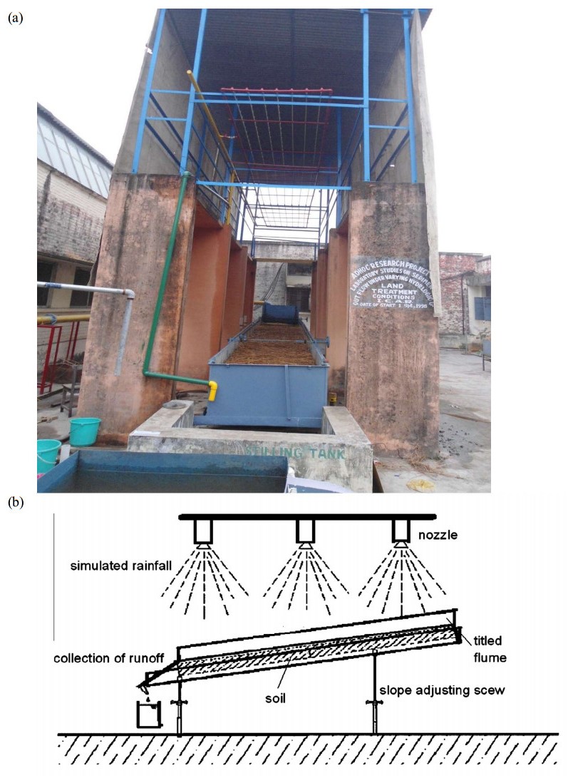
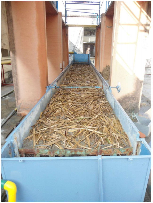
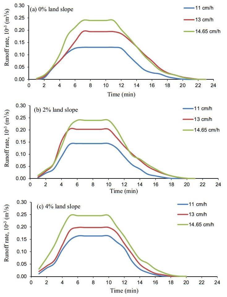
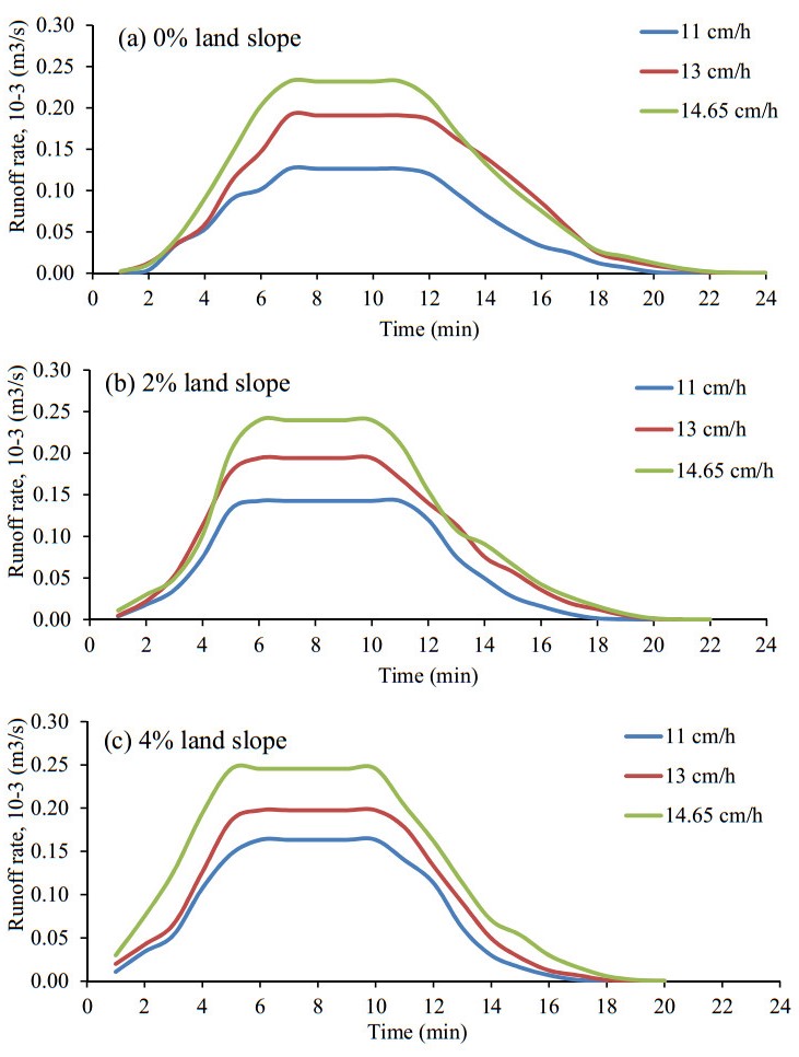
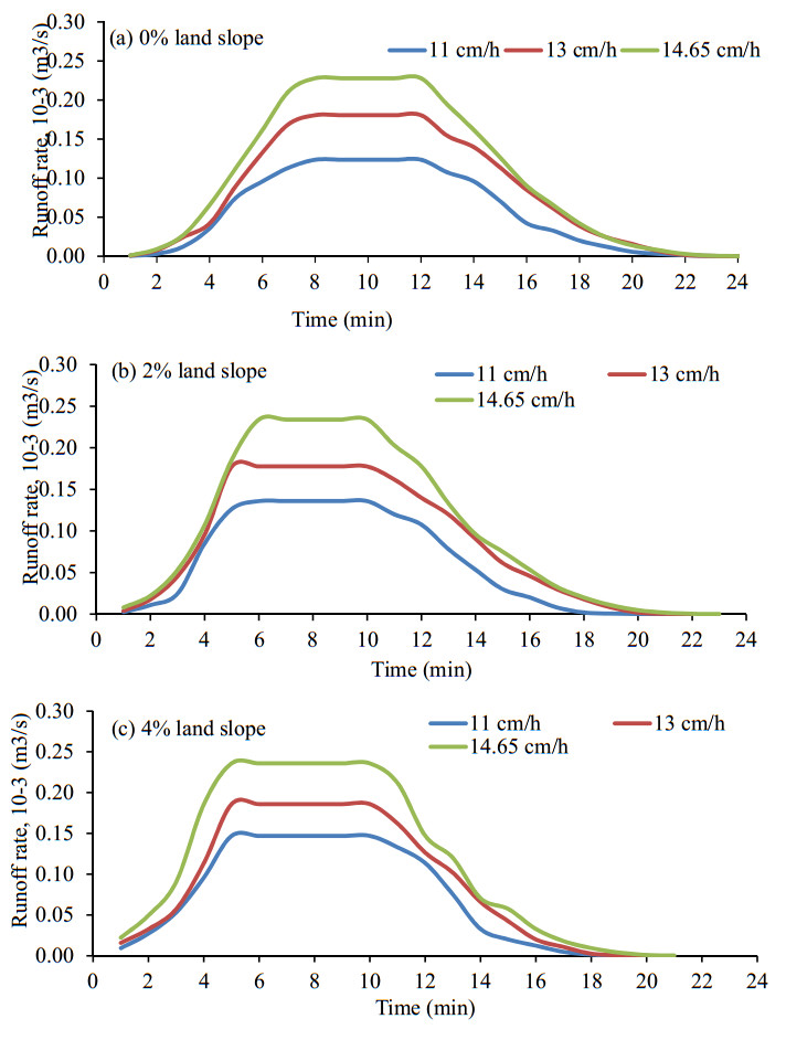
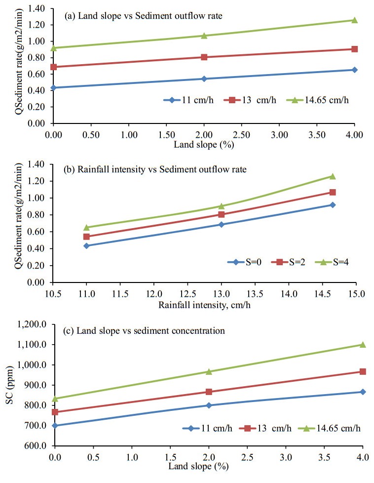
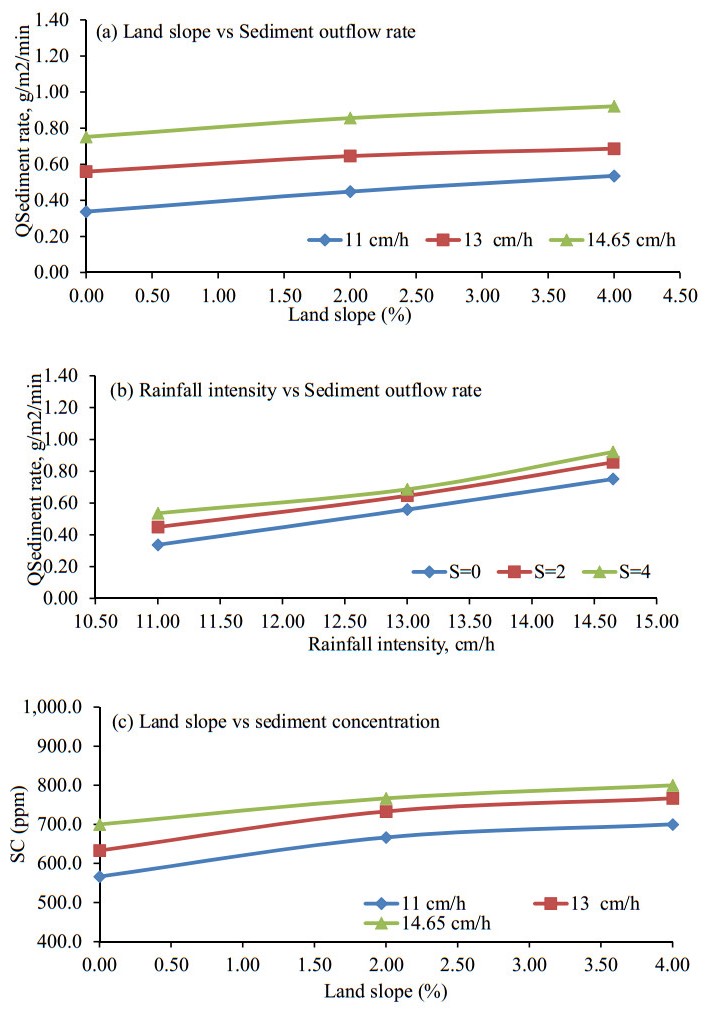
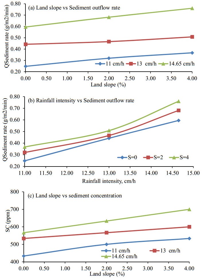
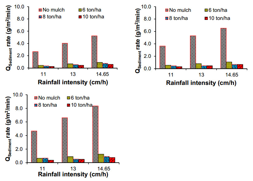
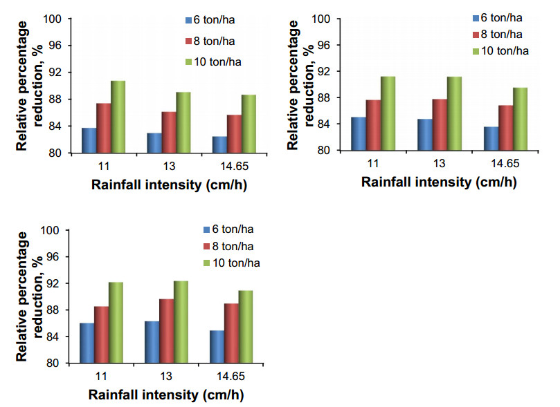
Trash mulches are remarkably effective in preventing soil erosion, reducing runoff-sediment transport-erosion, and increasing infiltration. The study was carried out to observe the sediment outflow from sugar cane leaf (trash) mulch treatments at selected land slopes under simulated rainfall conditions using a rainfall simulator of size 10 m × 1.2 m × 0.5 m with the locally available soil material collected from Pantnagar. In the present study, trash mulches with different quantities were selected to observe the effect of mulching on soil loss reduction. The number of mulches was taken as 6, 8 and 10 t/ha, three rainfall intensities viz. 11, 13 and 14.65 cm/h at 0, 2 and 4% land slopes were selected. The rainfall duration was fixed (10 minutes) for every mulch treatment. The total runoff volume varied with mulch rates for constant rainfall input and land slope. The average sediment concentration (SC) and sediment outflow rate (SOR) increased with the increasing land slope. However, SC and outflow decreased with the increasing mulch rate for a fixed land slope and rainfall intensity. The SOR for no mulch-treated land was higher than trash mulch-treated lands. Mathematical relationships were developed for relating SOR, SC, land slope, and rainfall intensity for a particular mulch treatment. It was observed that SOR and average SC values correlated with rainfall intensity and land slope for each mulch treatment. The developed models' correlation coefficients were more than 90%.
Citation: Sachin Kumar Singh, Dinesh Kumar Vishwakarma, Salwan Ali Abed, Nadhir Al-Ansari, P. S. Kashyap, Akhilesh Kumar, Pankaj Kumar, Rohitashw Kumar, Rajkumar Jat, Anuj Saraswat, Alban Kuriqi, Ahmed Elbeltagi, Salim Heddam, Sungwon Kim. Soil erosion control from trash residues at varying land slopes under simulated rainfall conditions[J]. Mathematical Biosciences and Engineering, 2023, 20(6): 11403-11428. doi: 10.3934/mbe.2023506
Trash mulches are remarkably effective in preventing soil erosion, reducing runoff-sediment transport-erosion, and increasing infiltration. The study was carried out to observe the sediment outflow from sugar cane leaf (trash) mulch treatments at selected land slopes under simulated rainfall conditions using a rainfall simulator of size 10 m × 1.2 m × 0.5 m with the locally available soil material collected from Pantnagar. In the present study, trash mulches with different quantities were selected to observe the effect of mulching on soil loss reduction. The number of mulches was taken as 6, 8 and 10 t/ha, three rainfall intensities viz. 11, 13 and 14.65 cm/h at 0, 2 and 4% land slopes were selected. The rainfall duration was fixed (10 minutes) for every mulch treatment. The total runoff volume varied with mulch rates for constant rainfall input and land slope. The average sediment concentration (SC) and sediment outflow rate (SOR) increased with the increasing land slope. However, SC and outflow decreased with the increasing mulch rate for a fixed land slope and rainfall intensity. The SOR for no mulch-treated land was higher than trash mulch-treated lands. Mathematical relationships were developed for relating SOR, SC, land slope, and rainfall intensity for a particular mulch treatment. It was observed that SOR and average SC values correlated with rainfall intensity and land slope for each mulch treatment. The developed models' correlation coefficients were more than 90%.

| [1] |
A. Kumawat, D. Yadav, P. Srivastava, D. Kumar, Restoration of agroecosystems with conservation agriculture for food security to achieve sustainable development goals, Land Degrad. Dev., 2023 (2023), 1–9. https://doi.org/10.1002/ldr.4677 doi: 10.1002/ldr.4677

|
| [2] |
S. Ullah, A. Ali, M. Iqbal, Z. A. Kazmi, M. Sodangi, R. F. Tufail, et al., Geospatial assessment of soil erosion intensity and sediment yield: a case study of Potohar Region, Environ. Earth Sci., 77 (2018), 705. https://doi.org/10.1007/s12665-018-7867-7 doi: 10.1007/s12665-018-7867-7
|
| [3] |
D. Pimentel, Soil erosion: A food and environmental threat, Environ. Dev. Sustain., 8 (2006), 119–137. https://doi.org/10.1007/s10668-005-1262-8 doi: 10.1007/s10668-005-1262-8
|
| [4] | M. Ashraf, K. Fayyaz-ul-Hussan, Sustainable environment management: impact of Agriculture, Sci. Technol. Dev., 19 (2000), 51–57. |
| [5] |
P. R. Hobbs, Conservation agriculture: what is it and why is it important for future sustainable food production?, J. Agric. Sci., 145 (2007), 127. https://doi.org/10.1017/S0021859607006892 doi: 10.1017/S0021859607006892
|
| [6] | Z. Shah, M. Arshad, Land degradation in Pakistan: a serious threat to environments and economic sustainability, 2006 (2006). |
| [7] |
S. A. Khresat, Z. Rawajfih, M. Mohammad, Land degradation in north-western Jordan: causes and processes, J. Arid. Environ., 39 (1998), 623–629. https://doi.org/10.1006/jare.1998.0385 doi: 10.1006/jare.1998.0385
|
| [8] | O. A. Abdi, E. K. Glover, O. Luukkanen, Causes and impacts of land degradation and desertification: Case study of the Sudan, Int. J. A gricul., 3 (2013), 40–51. |
| [9] |
H. Eswaran, R. Lal, P. F. Reich, Land degradation: an overview, Resp. Degrad., 2001 (2001), 20–35. https://doi.org/10.1201/9780429187957-4 doi: 10.1201/9780429187957-4
|
| [10] |
R. Lal, Restoring soil quality to mitigate soil degradation, Sustainability, 7 (2015), 5875–5895. https://doi.org/10.3390/su7055875 doi: 10.3390/su7055875
|
| [11] |
R. Lal, Soil erosion and the global carbon budget, Environ. Int., 29 (2003), 437–450. https://doi.org/10.1016/S0160-4120(02)00192-7 doi: 10.1016/S0160-4120(02)00192-7
|
| [12] | M. Ashraf, F. U. Hassan, A. Saleem, M. M. Iqbal, Soil conservation and management: A prerequisite for sustainable agriculture in pothwar, Sci. Technol. Dev., 21 (2002), 25–31. |
| [13] |
D. Pimentel, M. Burgess, Soil erosion threatens food production, Agriculture, 3 (2013), 443–463. https://doi.org/10.3390/agriculture3030443 doi: 10.3390/agriculture3030443
|
| [14] |
H. Aytop, S. Şenol, The effect of different land use planning scenarios on the amount of total soil losses in the Mikail Stream Micro-Basin, Environ. Monit. Assess, 194 (2022), 321. https://doi.org/10.1007/s10661-022-09937-2 doi: 10.1007/s10661-022-09937-2
|
| [15] | L. Tsegaye, R. Bharti, Assessment of the effects of agricultural management practices on soil erosion and sediment yield in Rib watershed, Ethiopia, Int. J. Environ. Sci. Technol., 2022 (2022). https://doi.org/10.1007/s13762-022-04018-w |
| [16] | D. Mandal, V. N. Sharda, Assessment of permissible soil loss in India employing a quantitative bio-physical model, Curr. Sci., 100 (2011), 383–390. |
| [17] | S. Kumar, J. G. Kalambukattu, Modeling and Monitoring Soil Erosion by Water Using Remote Sensing Satellite Data and GIS BT-Anthropogeomorphology: A Geospatial Technology Based Approach, Cham, Springer International Publishing, 2022. https://doi.org/10.1007/978-3-030-77572-8_14 |
| [18] | T. Svoray, The Case of Agricultural Catchments BT-A Geoinformatics Approach to Water Erosion: Soil Loss and Beyond, Cham, Springer International Publishing, 2022. https://doi.org/10.1007/978-3-030-91536-0 |
| [19] |
Y. Su, Y. Zhang, H. Wang, N. Lei, P. Li, J. Wang, Interactive effects of rainfall intensity and initial thaw depth on slope erosion, Sustainability, 14 (2022), 3172. https://doi.org/10.3390/su14063172 doi: 10.3390/su14063172
|
| [20] | Y. Li, X. Lu, R. A. Washington-Allen, Y. Li, Microtopographic controls on erosion and deposition of a rilled hillslope in eastern tennessee, USA, Remote Sens., 14 (2022), 1315. https://doi.org/10.3390/rs14061315 |
| [21] | W. H. Wischmeier, D. D. Smith, Predicting rainfall-erosion losses from cropland east of the Rocky Mountains: Guide for selection of practices for soil and water conservation, in Agricultural Research Service, US Department of Agriculture, (1965). |
| [22] | R. Cruse, D. Flanagan, J. Frankenberger, B. Gelder, D. Herzmann, D. James, et al., Daily estimates of rainfall, water runoff, and soil erosion in Iowa, J. Soil Water Conserv., 61 (2006), 191–199. |
| [23] | V. Prasannakumar, H. Vijith, S. Abinod, N. Geetha, Estimation of soil erosion risk within a small mountainous sub-watershed in Kerala, India, using Revised Universal Soil Loss Equation (RUSLE) and geo-information technology, Geosci. Front., 3 (2012), 209–215. https://doi.org/10.1016/j.gsf.2011.11.003 |
| [24] |
N. Kayet, K. Pathak, A. Chakrabarty, S. Sahoo, Evaluation of soil loss estimation using the RUSLE model and SCS-CN method in hillslope mining areas, Int. Soil Water Conserv. Res., 6 (2018), 31–42. https://doi.org/10.1016/j.iswcr.2017.11.002 doi: 10.1016/j.iswcr.2017.11.002
|
| [25] |
R. B. Bryan, Soil erodibility and processes of water erosion on hillslope, Geomorphology, 32 (2000), 385–415. https://doi.org/10.1016/S0169-555X(99)00105-1 doi: 10.1016/S0169-555X(99)00105-1
|
| [26] |
H. Aksoy, M. L. Kavvas, A review of hillslope and watershed scale erosion and sediment transport models. CATENA, 64 (2005), 247–271. https://doi.org/10.1016/j.catena.2005.08.008 doi: 10.1016/j.catena.2005.08.008
|
| [27] |
M. Mahmoodabadi, S. A. Sajjadi, Effects of rain intensity, slope gradient and particle size distribution on the relative contributions of splash and wash loads to rain-induced erosion, Geomorphology, 253 (2016), 159–167. https://doi.org/10.1016/j.geomorph.2015.10.010 doi: 10.1016/j.geomorph.2015.10.010
|
| [28] |
J. Lu, F. Zheng, G. Li, F. Bian, J. An, The effects of raindrop impact and runoff detachment on hillslope soil erosion and soil aggregate loss in the Mollisol region of Northeast China, Soil Tillage Res., 161 (2016), 79–85. https://doi.org/10.1016/j.still.2016.04.002 doi: 10.1016/j.still.2016.04.002
|
| [29] |
L. D. Meyer, W. H. Wischmeier, Mathematical simulation of the process of soil erosion by water, Trans. ASAE, 12 (1969), 754–758. https://doi.org/10.13031/2013.38945 doi: 10.13031/2013.38945
|
| [30] |
G. R. Foster, R. A. Young, M. J. M. Römkens, C. A. Onstad, Processes of soil erosion by water. Soil Eros Crop. Prod., 1985 (1985), 137–162. https://doi.org/10.2134/1985.soilerosionandcrop.c9 doi: 10.2134/1985.soilerosionandcrop.c9
|
| [31] |
T. Smets, J. Poesen, R. Bhattacharyya, M. A. Fullen, M. Subedi, C. A. Booth, et al., Evaluation of biological geotextiles for reducing runoff and soil loss under various environmental conditions using laboratory and field plot data, Land Degrad. Dev., 22 (2011), 480–494. https://doi.org/10.1002/ldr.1095 doi: 10.1002/ldr.1095
|
| [32] | L. Ferreras, E. Gomez, S. Toresani, I. Firpo, R. Rotondo, Effect of organic amendments on some physical, chemical and biological properties in a horticultural soil, Bioresour. Technol., 97 (2006), 635–640. https://doi.org/10.1016/j.biortech.2005.03.018 |
| [33] |
K. S. Rawat, S. K. Singh, Appraisal of soil conservation capacity using NDVI Model-based c factor of RUSLE Model for a semi arid ungauged watershed: a case study, Water Conserv. Sci. Eng., 3 (2018), 47–58. https://doi.org/10.1007/s41101-018-0042-x doi: 10.1007/s41101-018-0042-x
|
| [34] |
P. Zhou, O. Luukkanen, T. Tokola, J. Nieminen, Effect of vegetation cover on soil erosion in a mountainous watershed, CATENA, 75 (2008), 319–325. https://doi.org/10.1016/j.catena.2008.07.010 doi: 10.1016/j.catena.2008.07.010
|
| [35] | J. D. R. Sinoga, A. R. Diaz, F. E. Bueno, J. F. M. Murillo, The role of soil surface conditions in regulating runoff and erosion processes on a metamorphic hillslope (Southern Spain): Soil surface conditions, runoff and erosion in Southern Spain, CATENA, 80 (2010), 131–139. https://doi.org/10.1016/j.catena.2009.09.007 |
| [36] | L. Gholami, S. H. Sadeghi, M. Homaee, Straw mulching effect on splash erosion, runoff, and sediment yield from eroded plots, Soil Sci. Soc. Am. J., 77 (2013), 268–278. https://doi.org/10.2136/sssaj2012.0271 |
| [37] |
S. H. R. Sadeghi, L. Gholami, E. Sharifi, A. K. Darvishan, M. Homaee, Scale effect on runoff and soil loss control using rice straw mulch under laboratory conditions, Solid. Earth, 6 (2015), 1–8. https://doi.org/10.5194/se-6-1-2015 doi: 10.5194/se-6-1-2015
|
| [38] |
T. Smets, J. Poesen, A. Knapen, Spatial scale effects on the effectiveness of organic mulches in reducing soil erosion by water, Earth Sci. Rev., 89 (2008), 1–12. https://doi.org/10.1016/j.earscirev.2008.04.001 doi: 10.1016/j.earscirev.2008.04.001
|
| [39] |
N. K. Fageria, Role of soil organic matter in maintaining sustainability of cropping systems, Commun. Soil Sci. Plant Anal., 43 (2012), 2063–2113. https://doi.org/10.1080/00103624.2012.697234 doi: 10.1080/00103624.2012.697234
|
| [40] |
S. E. Obalum, G. U. Chibuike, S. Y. Peth, Ouyang, Soil organic matter as sole indicator of soil degradation, Environ. Monit. Assess., 189 (2017), 176. https://doi.org/10.1007/s10661-017-5881-y doi: 10.1007/s10661-017-5881-y
|
| [41] |
Z. H. Shi, B. J. Yue, L. Wang, N. F. Fang, D. Wang, F. Z. Wu, Effects of mulch cover rate on interrill erosion processes and the size selectivity of eroded sediment on steep slopes, Soil Sci. Soc. Am. J., 77 (2013), 257–267. https://doi.org/10.2136/sssaj2012.0273 doi: 10.2136/sssaj2012.0273
|
| [42] |
T. Guo, Q. Wang, D. Li, J. Zhuang, Effect of surface stone cover on sediment and solute transport on the slope of fallow land in the semi-arid loess region of northwestern China, J. Soils Sediments, 10 (2010), 1200–1208. https://doi.org/10.1007/s11368-010-0257-8 doi: 10.1007/s11368-010-0257-8
|
| [43] |
M. Prosdocimi, A. Jordán, P. Tarolli, S. Keesstra, A. Novara, A. Cerdà, The immediate effectiveness of barley straw mulch in reducing soil erodibility and surface runoff generation in Mediterranean vineyards, Sci. Total Environ., 547 (2016), 323–330. https://doi.org/10.1016/j.scitotenv.2015.12.076 doi: 10.1016/j.scitotenv.2015.12.076
|
| [44] |
A. A. A. Montenegro, J. R. C. B. Abrantes, J. L. M. P. de Lima, V. P. Singh, T. E. M. Santos, Impact of mulching on soil and water dynamics under intermittent simulated rainfall, CATENA., 109 (2013), 139–149. https://doi.org/10.1016/j.catena.2013.03.018 doi: 10.1016/j.catena.2013.03.018
|
| [45] | A. D. Abrahams, A. J. Parsons, Relation between infiltration and stone cover on a semiarid hillslope, southern Arizona, J. Hydrol., 122 (1991), 49–59. https://doi.org/10.1016/0022-1694(91)90171-D |
| [46] |
C. Valentin, A. Casenave, Infiltration into sealed soils as influenced by gravel cover, Soil Sci. Soc. Am. J., 56 (1992), 1667–1673. https://doi.org/10.2136/sssaj1992.03615995005600060002x doi: 10.2136/sssaj1992.03615995005600060002x
|
| [47] |
J. W. Poesen, D. Torri, K. Bunte, Effects of rock fragments on soil erosion by water at different spatial scales: a review, CATENA, 23 (1994), 141–166. https://doi.org/10.1016/0341-8162(94)90058-2 doi: 10.1016/0341-8162(94)90058-2
|
| [48] | A. Cerdà, Effects of rock fragment cover on soil infiltration, interrill runoff and erosion, Eur. J. Soil Sci., 52 (2001), 59–68. https://doi.org/10.1046/j.1365-2389.2001.00354.x |
| [49] |
L. M. Zavala, A. Jordán, N. Bellinfante, J. Gill, Relationships between rock fragment cover and soil hydrological response in a Mediterranean environment, Soil Sci. Plant Nutr., 56 (2010), 95–104. https://doi.org/10.1111/j.1747-0765.2009.00429.x doi: 10.1111/j.1747-0765.2009.00429.x
|
| [50] |
R. Akis, R. Lal, Evaluation of seasonal effects of tillage and drainage management practices on soil physical properties and infiltration characteristics in a silt-loam soil, Eur. J. Sci. Technol., 2022 (2022), 1011–1023. https://doi.org/10.31590/ejosat.1050860 doi: 10.31590/ejosat.1050860
|
| [51] |
Molla A, Desta G, Molla GA, Soil management and crop practice effect on soil water infiltration and soil water storage in the humid Lowlands of Beles Sub-Basin, Ethiopia, Hydrology, 10 (2022), 1–11. https://doi.org/10.11648/j.hyd.20221001.11 doi: 10.11648/j.hyd.20221001.11
|
| [52] |
K. O. Adekalu, I. A. Olorunfemi, J. A. Osunbitan, Grass mulching effect on infiltration, surface runoff and soil loss of three agricultural soils in Nigeria, Bioresour. Technol., 98 (2007), 912–917. https://doi.org/10.1016/j.biortech.2006.02.044 doi: 10.1016/j.biortech.2006.02.044
|
| [53] |
C. Pan, Z. Shangguan, Runoff hydraulic characteristics and sediment generation in sloped grassplots under simulated rainfall conditions, J. Hydrol., 331 (2006), 178–185. https://doi.org/10.1016/j.jhydrol.2006.05.011 doi: 10.1016/j.jhydrol.2006.05.011
|
| [54] |
C. Pan, L. Ma, Z. Shangguan, Effectiveness of grass strips in trapping suspended sediments from runoff, Earth Surf. Process Landforms, 35 (2010), 1006–1013. https://doi.org/10.1002/esp.1997 doi: 10.1002/esp.1997
|
| [55] |
R. Bhattacharyya, T. Smets, M. A. Fullen, J. Poesen, C.A. Booth, Effectiveness of geotextiles in reducing runoff and soil loss: A synthesis, CATENA, 81 (2010), 184–195. https://doi.org/10.1016/j.catena.2010.03.003 doi: 10.1016/j.catena.2010.03.003
|
| [56] |
A. Cerdà, S. H. Doerr. The effect of ash and needle cover on surface runoff and erosion in the immediate post-fire period, CATENA., 74 (2008), 256–263. https://doi.org/10.1016/j.catena.2008.03.010 doi: 10.1016/j.catena.2008.03.010
|
| [57] |
P. R. Robichaud, S. A. Lewis, J. W. Wagenbrenner, L. E. Ashmun, R. E. Brown, Post-fire mulching for runoff and erosion mitigation: Part I: Effectiveness at reducing hillslope erosion rates, CATENA, 105 (2013), 75–92. https://doi.org/10.1016/j.catena.2012.11.015 doi: 10.1016/j.catena.2012.11.015
|
| [58] |
P. R. Robichaud, J. W. Wagenbrenner, S. A. Lewis, L. E. Ashmun, R. E. Brown, P. M. Wohlgemuth, Post-fire mulching for runoff and erosion mitigation Part Ⅱ: Effectiveness in reducing runoff and sediment yields from small catchments, CATENA, 105 (2013), 93–111. https://doi.org/10.1016/j.catena.2012.11.016 doi: 10.1016/j.catena.2012.11.016
|
| [59] |
T. H. Dao, Tillage and winter wheat residue management effects on water infiltration and storage, Soil Sci. Soc. Am. J., 57 (1993), 1586–1595. https://doi.org/10.2136/sssaj1993.03615995005700060032x doi: 10.2136/sssaj1993.03615995005700060032x
|
| [60] |
P. Govindasamy, J. Mowrer, N. Rajan, T. Provin, F. Hons, M. Bagavathiannan, Influence of long-term (36 years) tillage practices on soil physical properties in a grain sorghum experiment in Southeast Texas, Arch. Agron. Soil Sci., 67 (2021), 234–244. https://doi.org/10.1080/03650340.2020.1720914 doi: 10.1080/03650340.2020.1720914
|
| [61] |
Y. Wang, J. Qiao, W. Ji, J. Sun, D. Huo, Y. Liu, et al., Effects of crop residue managements and tillage practices on variations of soil penetration resistance in sloping farmland of Mollisols, Int. J. Agric. Biol. Eng., 14 (2021), 164–171. https://doi.org/10.25165/j.ijabe.20221501.6526 doi: 10.25165/j.ijabe.20221501.6526
|
| [62] |
L. Benkobi, M. J. Trlica, J. L. Smith, Soil loss as affected by different combinations of surface litter and rock, J. Environ. Qual., 22 (1993), 657–661. https://doi.org/10.2134/jeq1993.00472425002200040003x doi: 10.2134/jeq1993.00472425002200040003x
|
| [63] |
H. J. Schmalz, R. V. Taylor, T. N. Johnson, P. L. Kennedy, S. J. DeBano, B. A. Newingham, et al., Soil morphologic properties and cattle stocking rate affect dynamic soil properties, Rangel. Ecol. Manage., 66 (2013), 445–453. https://doi.org/10.2111/REM-D-12-00040.1 doi: 10.2111/REM-D-12-00040.1
|
| [64] |
X. Li, J. Niu, B. Xie, The effect of leaf litter cover on surface runoff and soil erosion in Northern China, PLoS One, 9 (2014), e107789. https://doi.org/10.1371/journal.pone.0107789 doi: 10.1371/journal.pone.0107789
|
| [65] |
M. A. Weltz, M. R. Kidwell, H. D. Fox, Influence of abiotic and biotic factors in measuring and modeling soil erosion on rangelands: State of knowledge, J. Range Manage., 51 (1998), 482–495. https://doi.org/10.2307/4003363 doi: 10.2307/4003363
|
| [66] |
Y. Xin, Y. Xie, Y. Liu, X. Ren, Residue cover effects on soil erosion and the infiltration in black soil under simulated rainfall experiments, J. Hydrol., 543 (2016), 651–658. https://doi.org/10.1016/j.jhydrol.2016.10.036 doi: 10.1016/j.jhydrol.2016.10.036
|
| [67] | F. L. Engel, I. Bertol, S. R. Ritter, A. P. González, J. P. Ferreiro, E. Vidal Vázquez, Soil erosion under simulated rainfall in relation to phenological stages of soybeans and tillage methods in Lages, SC, Brazil, Soil Tillage Res., 103 (2009), 216–221. https://doi.org/10.1016/j.still.2008.05.017 |
| [68] |
J. R. C. B. Abrantes, S. A. Prats, J. J. Keizer, J. L. M. P. de Lima, Effectiveness of the application of rice straw mulching strips in reducing runoff and soil loss: Laboratory soil flume experiments under simulated rainfall, Soil Tillage Res., 180 (2018), 238–249. https://doi.org/10.1016/j.still.2018.03.015 doi: 10.1016/j.still.2018.03.015
|
| [69] |
D. R. Mailapalli, M. Burger, W. R. Horwath, W. W. Wallender, (2013) Crop residue biomass effects on agricultural runoff, Appl. Environ. Soil Sci., 2013 (2013), 1–8. https://doi.org/10.1155/2013/805206 doi: 10.1155/2013/805206
|
| [70] |
X. Liu, S. Zhang, X. Zhang, G. Ding, R. M. Cruse, Soil erosion control practices in Northeast China: A mini-review, Soil Tillage Res., 117 (2011), 44–48. https://doi.org/10.1016/j.still.2011.08.005 doi: 10.1016/j.still.2011.08.005
|
| [71] |
J. H. Zonta, M. A. Martinez, F. F. Pruski, D. D. Silva, M. R. Santos, Effect of successive rainfall with different patterns on soil water infiltration rate, Rev. Bras Ciência Solo, 36 (2012), 377–388. https://doi.org/10.1590/S0100-06832012000200007 doi: 10.1590/S0100-06832012000200007
|
| [72] |
S. A. Prats, J. R. Abrantes, I. P. Crema, J. J. Keizer, J. L. M. P. Lima, Runoff and soil erosion mitigation with sieved forest residue mulch strips under controlled laboratory conditions, Forest Ecol. Manage., 396 (2017), 102–112. https://doi.org/10.1016/j.foreco.2017.04.019 doi: 10.1016/j.foreco.2017.04.019
|
| [73] | S. A. Prats, M. A. Martins, M. C. Malvar, M. Ben-Hur, J. J. Keizer, Polyacrylamide application versus forest residue mulching for reducing post-fire runoff and soil erosion, Sci. Total Environ., 468–469 (2014), 464–474. https://doi.org/10.1016/j.scitotenv.2013.08.066 |
| [74] |
S. A. Prats, M. C. Malvar, D. C. S. Vieira, L. MacDonald, J. J. Keizer, Effectiveness of hydromulching to reduce runoff and erosion in a recently burnt pine plantation in central portugal, Land Degrad. Dev., 27 (2013), 1319–1333. https://doi.org/10.1002/ldr.2236 doi: 10.1002/ldr.2236
|
| [75] |
S. A. Prats, L. H. MacDonald, M. Monteiro, A. J. D. Ferreira, C. O. A. Coelho, J. J. Keizer, Effectiveness of forest residue mulching in reducing post-fire runoff and erosion in a pine and a eucalypt plantation in north-central Portugal, Geoderma, 191 (2012), 115–124. https://doi.org/10.1016/j.geoderma.2012.02.009 doi: 10.1016/j.geoderma.2012.02.009
|
Figures(10) / Tables(3)

Sachin Kumar Singh, Dinesh Kumar Vishwakarma, Salwan Ali Abed, Nadhir Al-Ansari, P. S. Kashyap, Akhilesh Kumar, Pankaj Kumar, Rohitashw Kumar, Rajkumar Jat, Anuj Saraswat, Alban Kuriqi, Ahmed Elbeltagi, Salim Heddam, Sungwon Kim. Soil erosion control from trash residues at varying land slopes under simulated rainfall conditions[J]. Mathematical Biosciences and Engineering, 2023, 20(6): 11403-11428. doi: 10.3934/mbe.2023506


 DownLoad: