Semi-supervised regression with adaptive graph learning for EEG-based emotion recognition

Tianhui Sha; Yikai Zhang; Yong Peng; Wanzeng Kong; Tianhui Sha; Yikai Zhang; Yong Peng; Wanzeng Kong

doi:10.3934/mbe.2023505

Mathematical Biosciences and Engineering

2023, Volume 20, Issue 6: 11379-11402. doi: 10.3934/mbe.2023505

Previous Article Next Article

Research article

Semi-supervised regression with adaptive graph learning for EEG-based emotion recognition

1.
School of Computer Science and Technology, Hangzhou Dianzi University, Hangzhou, 310018, China
2.
Zhejiang Key Laboratory of Brain-Machine Collaborative Intelligence, Hangzhou, 310018, China

Received: 12 March 2023 Revised: 16 April 2023 Accepted: 18 April 2023 Published: 27 April 2023

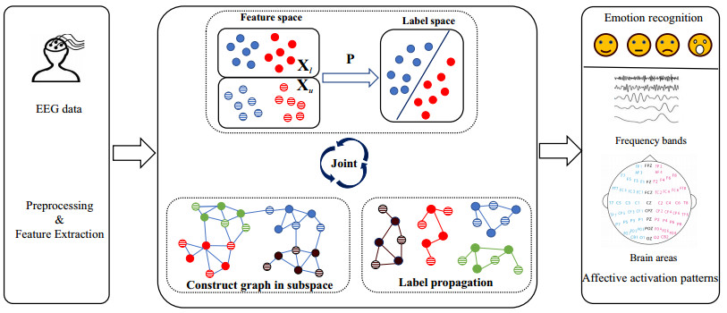
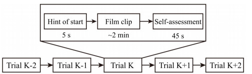
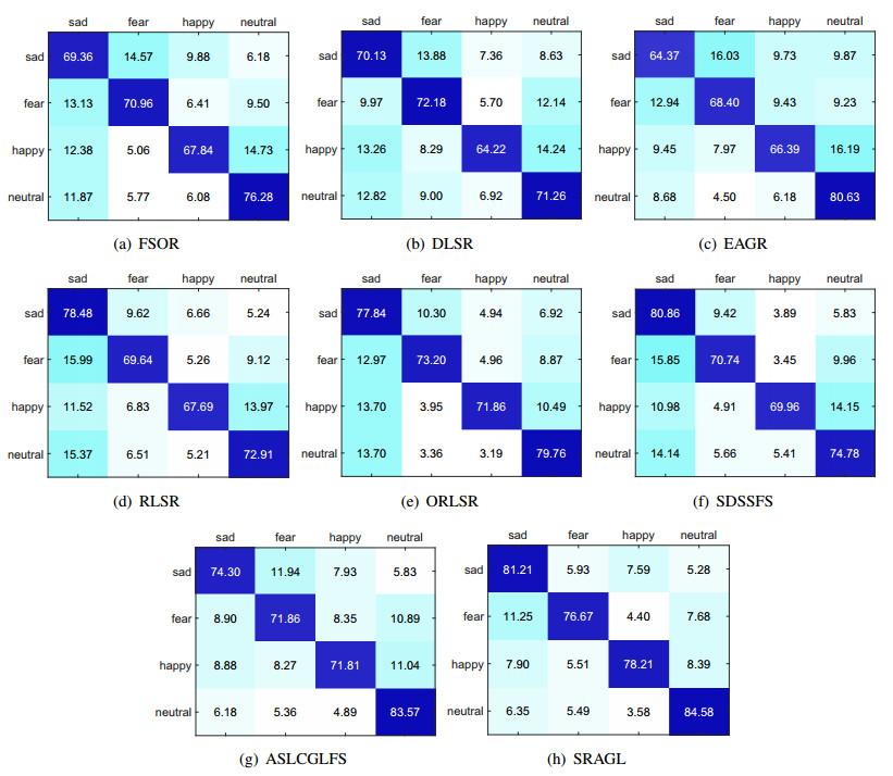
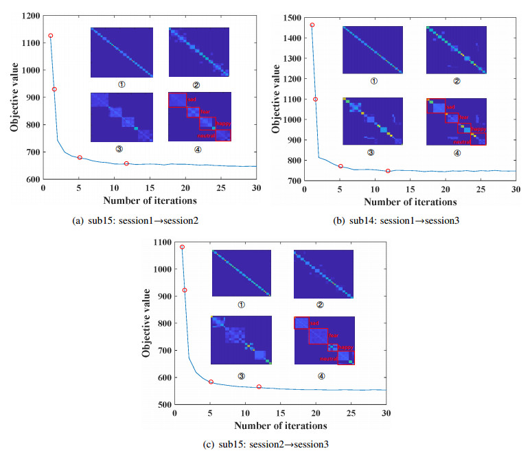
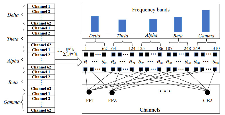
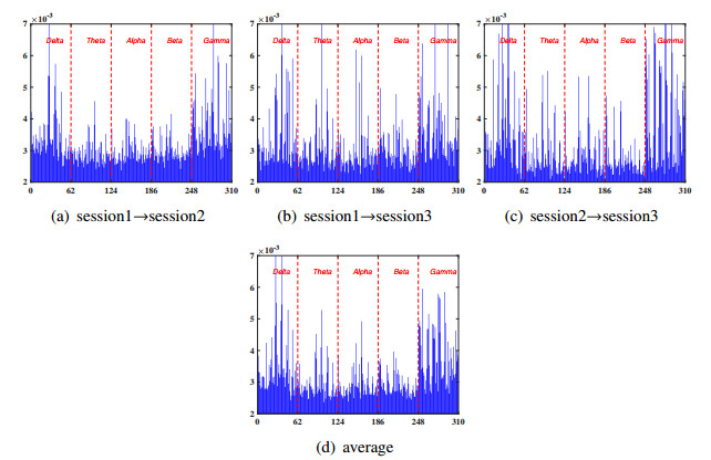
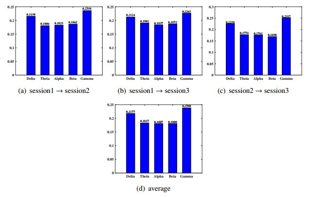
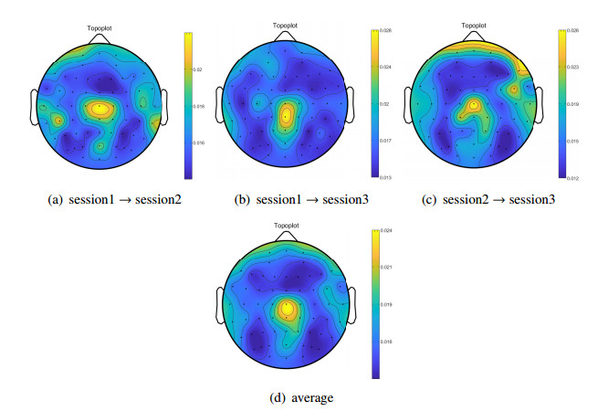
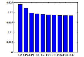
Electroencephalogram (EEG) signals are widely used in the field of emotion recognition since it is resistant to camouflage and contains abundant physiological information. However, EEG signals are non-stationary and have low signal-noise-ratio, making it more difficult to decode in comparison with data modalities such as facial expression and text. In this paper, we propose a model termed semi-supervised regression with adaptive graph learning (SRAGL) for cross-session EEG emotion recognition, which has two merits. On one hand, the emotional label information of unlabeled samples is jointly estimated with the other model variables by a semi-supervised regression in SRAGL. On the other hand, SRAGL adaptively learns a graph to depict the connections among EEG data samples which further facilitates the emotional label estimation process. From the experimental results on the SEED-IV data set, we have the following insights. 1) SRAGL achieves superior performance compared to some state-of-the-art algorithms. To be specific, the average accuracies are 78.18%, 80.55%, and 81.90% in the three cross-session emotion recognition tasks. 2) As the iteration number increases, SRAGL converges quickly and optimizes the emotion metric of EEG samples gradually, leading to a reliable similarity matrix finally. 3) Based on the learned regression projection matrix, we obtain the contribution of each EEG feature, which enables us to automatically identify critical frequency bands and brain regions in emotion recognition.
- adaptive graph learning,
- Electroencephalogram (EEG),
- emotion recognition,
- graph label propagation,
- semi-supervised regression
Citation: Tianhui Sha, Yikai Zhang, Yong Peng, Wanzeng Kong. Semi-supervised regression with adaptive graph learning for EEG-based emotion recognition[J]. Mathematical Biosciences and Engineering, 2023, 20(6): 11379-11402. doi: 10.3934/mbe.2023505

Related Papers:

Abstract

Electroencephalogram (EEG) signals are widely used in the field of emotion recognition since it is resistant to camouflage and contains abundant physiological information. However, EEG signals are non-stationary and have low signal-noise-ratio, making it more difficult to decode in comparison with data modalities such as facial expression and text. In this paper, we propose a model termed semi-supervised regression with adaptive graph learning (SRAGL) for cross-session EEG emotion recognition, which has two merits. On one hand, the emotional label information of unlabeled samples is jointly estimated with the other model variables by a semi-supervised regression in SRAGL. On the other hand, SRAGL adaptively learns a graph to depict the connections among EEG data samples which further facilitates the emotional label estimation process. From the experimental results on the SEED-IV data set, we have the following insights. 1) SRAGL achieves superior performance compared to some state-of-the-art algorithms. To be specific, the average accuracies are 78.18%, 80.55%, and 81.90% in the three cross-session emotion recognition tasks. 2) As the iteration number increases, SRAGL converges quickly and optimizes the emotion metric of EEG samples gradually, leading to a reliable similarity matrix finally. 3) Based on the learned regression projection matrix, we obtain the contribution of each EEG feature, which enables us to automatically identify critical frequency bands and brain regions in emotion recognition.

References

[1]	R. Adolphs, D. J Anderson, The neuroscience of emotion, In The Neuroscience of Emotion, Princeton University Press, 2018. https://doi.org/10.23943/9781400889914
[2]	Z, Halim, M, Rehan, On identification of driving-induced stress using electroencephalogram signals: A framework based on wearable safety-critical scheme and machine learning, Inform. Fusion, 53 (2020), 66–79. https://doi.org/10.1016/j.inffus.2019.06.006 doi: 10.1016/j.inffus.2019.06.006
[3]	H. Cai, Z. Qu, Z. Li, Y. Zhang, X. Hu, B. Hu, Feature-level fusion approaches based on multimodal EEG data for depression recognition, Inform. Fusion, 59 (2020), 2127–138. https://doi.org/10.1016/j.inffus.2020.01.008 doi: 10.1016/j.inffus.2020.01.008
[4]	D. Xu, X. Qin, X. Dong, X. Cui, Emotion recognition of EEG signals based on variational mode decomposition and weighted cascade forest, Math. Biosci. Eng, 20 (2023), 2566–2587. https://doi.org/10.3934/mbe.2023120 doi: 10.3934/mbe.2023120
[5]	J. Xue, J. Wang, S. Hu, N. Bi, Z. Lv, OVPD: odor-video elicited physiological signal database for emotion recognition, IEEE Trans. Instrum. Meas., 71 (2022), 1–12. https://doi.org/10.1109/TIM.2022.3149116 doi: 10.1109/TIM.2022.3149116
[6]	N. Suhaimi, J. Mountstephens, J. Teo, EEG-based emotion recognition: A state-of-the-art review of current trends and opportunities, Comput. Intel. Neurosc., 2020 (2020), 1–19. https://doi.org/10.1155/2020/8875426 doi: 10.1155/2020/8875426
[7]	Y. Ou, S. Sun, H. Gan, R. Zhou, Z. Yang, An improved self-supervised learning for EEG classification, Math. Biosci. Eng., 19 (2022), 6907–6922. https://doi.org/10.3934/mbe.2022325 doi: 10.3934/mbe.2022325
[8]	X. Li, D. Song, P. Zhang, Y. Zhang, Y. Hou, B Hu, Exploring EEG features in cross-subject emotion recognition, Front. Neurosci., 12 (2018), 162. https://doi.org/10.3389/fnins.2018.00162 doi: 10.3389/fnins.2018.00162
[9]	Y. Dan, J. Tao, J. Fu, D. Zhou, Possibilistic clustering-promoting semi-supervised learning for EEG-based emotion recognition, Front. Neurosci., 15 (2021), 690044. https://doi.org/10.3389/fnins.2021.690044 doi: 10.3389/fnins.2021.690044
[10]	X. Chen, L. Song, Y. Hou, G. Shao, Efficient semi-supervised feature selection for VHR remote sensing images, In Proc. IEEE Int. Geosci. Remote Sens. Symp., (2016), 1500–1503. https://doi.org/10.1109/IGARSS.2016.7729383
[11]	B. Tang, L. Zhang, Local preserving logistic i-relief for semi-supervised feature selection, Neurocomputing, 399 (2020), 48–64. https://doi.org/10.1016/j.neucom.2020.02.098 doi: 10.1016/j.neucom.2020.02.098
[12]	H. Gan, Z. Li, W. Wu, Z. Luo, R. Huang, Safety-aware graph-based semi-supervised learning, Expert Syst. Appl., 107 (2018), 243–254. https://doi.org/10.1016/j.eswa.2018.04.031 doi: 10.1016/j.eswa.2018.04.031
[13]	Y. Peng, Wa. Kong, F. Qin, F. Nie, Manifold adaptive kernelized low-rank representation for semisupervised image classification, Complexity, 2018 (2018), 1–12. https://doi.org/10.1155/2018/2857594 doi: 10.1155/2018/2857594
[14]	Z. Kang, Z. Lin, X. Zhu, W. Xu, Structured graph learning for scalable subspace clustering: From single view to multiview, IEEE Trans. Cybern., 52 (2021), 8976–8986. https://doi.org/10.1109/TCYB.2021.3061660 doi: 10.1109/TCYB.2021.3061660
[15]	Z. Liu, Z. Lai, W. Ou, K. Zhang, R. Zheng, Structured optimal graph based sparse feature extraction for semi-supervised learning, Signal Process., 170 (2020), 107456. https://doi.org/10.1016/j.sigpro.2020.107456 doi: 10.1016/j.sigpro.2020.107456
[16]	Z. Lin, Z. Kang, L. Zhang, L. Tian, Multi-view attributed graph clustering, IEEE Trans. Knowl. Data Eng., 35 (2021), 1872–1880. https://doi.org/10.1016/10.1109/TKDE.2021.3101227 doi: 10.1016/10.1109/TKDE.2021.3101227
[17]	F. Nie, Z. Wang, R. Wang, X. Li, Adaptive local embedding learning for semi-supervised dimensionality reduction, IEEE Trans. Knowl. Data En., 34 (2021), 4609–4621. https://doi.org/10.1109/TKDE.2021.3049371 doi: 10.1109/TKDE.2021.3049371
[18]	X. Chen, R. Chen, Q. Wu, F. Nie, M. Yang, R. Mao, Semisupervised feature selection via structured manifold learning, IEEE Trans. Cybern., 52 (2021), 5756–5766. https://doi.org/10.1109/TCYB.2021.3052847 doi: 10.1109/TCYB.2021.3052847
[19]	G. Haeser, M. Schuverdt, On approximate KKT condition and its extension to continuous variational inequalities, J. Optimiz. Theory App., 149 (2011), 528–539. https://doi.org/10.1007/s10957-011-9802-x doi: 10.1007/s10957-011-9802-x
[20]	Y. Peng, X. Zhu, F. Nie, W. Kong, Y. Ge, Fuzzy graph clustering, Inf. Sci., 571 (2021), 38–49. https://doi.org/10.1016/j.ins.2021.04.058 doi: 10.1016/j.ins.2021.04.058
[21]	W. Zheng, W. Liu, Y. Lu, B. Lu, A. Cichocki, Emotionmeter: A multimodal framework for recognizing human emotions, IEEE Trans. Cybern., 49 (2019), 1110–1122. https://doi.org/10.1109/TCYB.2018.2797176 doi: 10.1109/TCYB.2018.2797176
[22]	R. Duan, J. Zhu, B. Lu, Differential entropy feature for EEG-based emotion classification, In Proc. Int. IEEE/EMBS Conf. Neural Eng., (2013), 81–84. https://doi.org/10.1109/NER.2013.6695876
[23]	L. Shi, Y. Jiao, B. Lu, Differential entropy feature for EEG-based vigilance estimation, In Proc. Ann. Int. Conf. IEEE Eng. Med. Biol. Soc. (EMBC), (2013), 6627–6630. https://doi.org/10.1109/EMBC.2013.6611075
[24]	X. Wu, X. Xu, J. Liu, H. Wang, B. Hu, F. Nie, Supervised feature selection with orthogonal regression and feature weighting, IEEE Trans. Neural Netw. Learn. Syst., 32 (2020), 1831–1838. https://doi.org/10.1109/TNNLS.2020.2991336 doi: 10.1109/TNNLS.2020.2991336
[25]	S. Xiang, F. Nie, G. Meng, C. Pan, C. Zhang, Discriminative least squares regression for multiclass classification and feature selection, IEEE Trans. Neural Netw. Learn. Syst., 23 (2012), 1738–1754. https://doi.org/10.1109/TNNLS.2012.2212721 doi: 10.1109/TNNLS.2012.2212721
[26]	M. Wang, W. Fu, S. Hao, D. Tao, X Wu, Scalable semi-supervised learning by efficient anchor graph regularization, IEEE Trans. Knowl. Data Eng., 28 (2016), 1864–1877. https://doi.org/10.1109/TKDE.2016.2535367 doi: 10.1109/TKDE.2016.2535367
[27]	X. Chen, G. Yuan, F. Nie, J. Huang, Semi-supervised feature selection via rescaled linear regression, In Proc. Int. J. Conf. Artif. Intell., 2017 (2017), 1525–1531. https://doi.org/10.24963/ijcai.2017/211
[28]	C. Wang, X. Chen, G. Yuan, F. Nie, M. Yang, Semi-supervised feature selection with sparse discriminative least squares regression, IEEE Trans. Cybern., 52 (2022), 8413–8424. https://doi.org/10.1109/TCYB.2021.3060804 doi: 10.1109/TCYB.2021.3060804
[29]	J. Lai, H. Chen, W. Li, T. Li, J. Wan, Semi-supervised feature selection via adaptive structure learning and constrained graph learning, Knowl. Based Syst., 251 (2022), 109243. https://doi.org/10.1016/j.knosys.2022.109243 doi: 10.1016/j.knosys.2022.109243
[30]	Z. Ma, Z. Xie, T. Qiu, J. Cheng, Driving event-related potential-based speller by localized posterior activities: An offline study, Math. Biosci. Eng, 17 (2020) 789–801. https://doi.org/10.3934/mbe.2020041
[31]	F. Nie, X. Wang, H. Huang, Clustering and projected clustering with adaptive neighbors, In Proc. ACM SIGKDD Int. Conf. Knowl. Disc. Data Min., (2014) 977–986. https://doi.org/10.1145/2623330.2623726
[32]	F. Nie, X. Wang, M. Jordan, H. Huang, The constrained laplacian rank algorithm for graph-based clustering, In Proc. AAAI Conf. Artif. Intell., (2016), 1969–1976. https://doi.org/10.1609/aaai.v30i1.10302
[33]	J. Han, K. Xiong, F. Nie, Orthogonal and nonnegative graph reconstruction for large scale clustering, In Proc. Int. J. Conf. Artif. Intell., (2017), 1809–1815. https://doi.org/10.24963/ijcai.2017/251
[34]	F. Nie, H. Huang, X. Cai, C. Ding, Efficient and robust feature selection via joint $\ell_{2, 1}$-norms minimization, In International Conference on Neural Information Processing Systems., 23 (2010), 1813–1821. https://doi.org/10.24963/ijcai.2017/251
[35]	Y. Peng, F. Qin, W. Kong, Y. Ge, F. Nie, A. Cichocki, GFIL: A unified framework for the importance analysis of features, frequency bands and channels in EEG-based emotion recognition, IEEE Trans. Cogn. Develop. Syst., 14 (2022), 935–947. https://doi.org/10.1109/TCDS.2021.3082803 doi: 10.1109/TCDS.2021.3082803
[36]	Y. Peng, W. Kong, F. Qin, F. Nie, J. Fang, B. Lu, A. Cichocki, Self-weighted semi-supervised classification for joint EEG-based emotion recognition and affective activation patterns mining, IEEE Trans. Instrum. Meas., 70 (2021), 1–11. https://doi.org/10.1109/TIM.2021.3124056 doi: 10.1109/TIM.2021.3124056
[37]	Z. Chen, S. Duan, Y. Peng, EEG-based emotion recognition by retargeted semi-supervised regression with robust weights, Systems, 10 (2022), 236. https://doi.org/10.3390/systems10060236 doi: 10.3390/systems10060236
[38]	X. Li, F. Shen, Y. Peng, W. Kong, B. Lu, Efficient sample and feature importance mining in semi-supervised EEG emotion recognition, IEEE Trans. Circuits Syst. II, Exp. Briefs, 69 (2022), 3349–3353. https://doi.org/10.1109/TCSII.2022.3163141 doi: 10.1109/TCSII.2022.3163141
[39]	Y. Peng, H. Liu, J. Li, J. Huang, B. Lu, W. Kong, Cross-session emotion recognition by joint label-common and label-specific EEG features exploration, IEEE Trans. Neur. Syst. Reh. Eng., 31 (2022), 759–768. https://doi.org/10.1109/TNSRE.2022.3233109 doi: 10.1109/TNSRE.2022.3233109
[40]	Y. Peng, F Jin, W. Kong, F. Nie, B. Lu, A. Cichocki, Ogssl: A semi-supervised classification model coupled with optimal graph learning for EEG emotion recognition, IEEE Trans. Neur. Syst. Reh. Eng., 30 (2022), 1288–1297. https://doi.org/10.1109/TNSRE.2022.3175464 doi: 10.1109/TNSRE.2022.3175464

Reader Comments

Your name:*

Email:*
© 2023 the Author(s), licensee AIMS Press. This is an open access article distributed under the terms of the Creative Commons Attribution License (http://creativecommons.org/licenses/by/4.0)