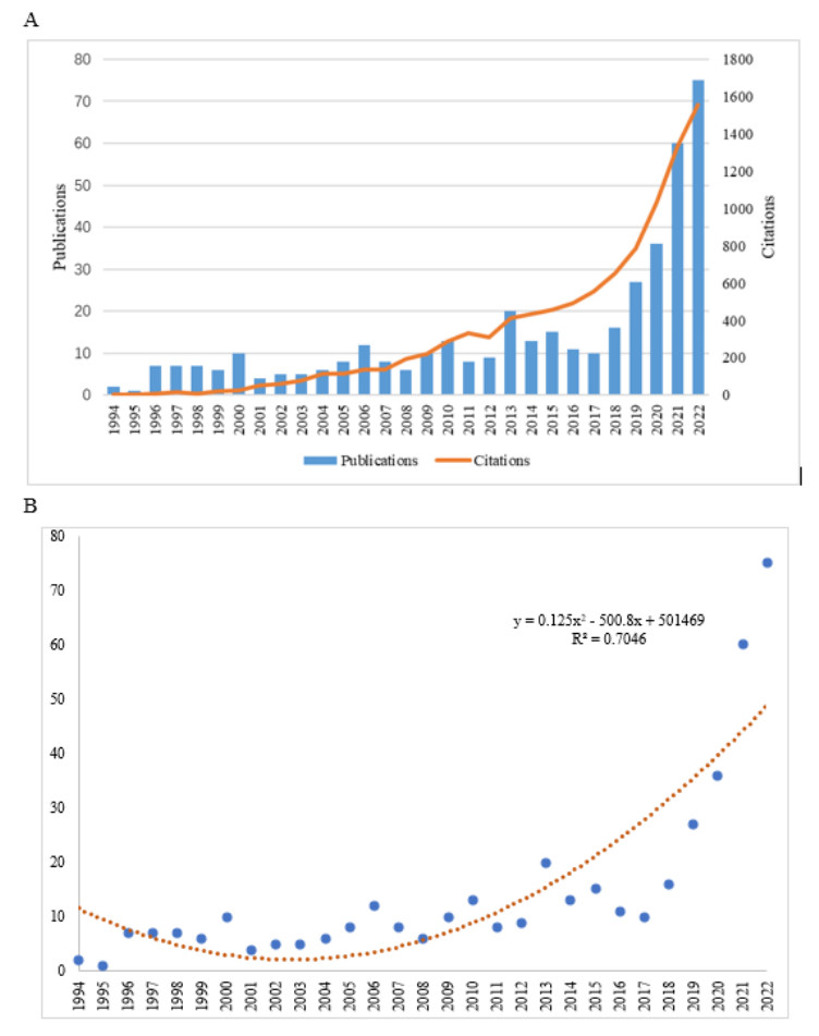
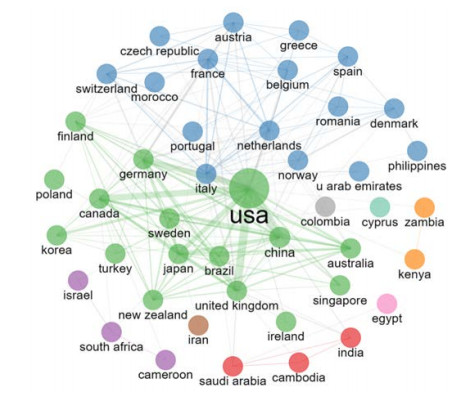
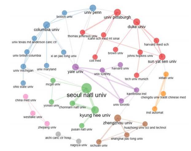
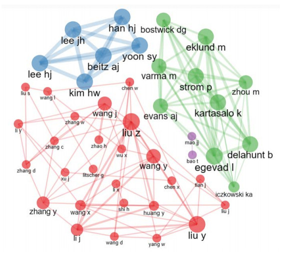
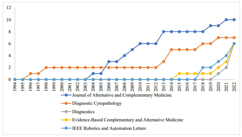
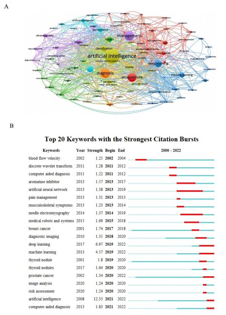
This study aimed to provide a panorama of artificial intelligence (AI) in acupuncture by characterizing and visualizing the knowledge structure, hotspots and trends in global scientific publications. Publications were extracted from the Web of Science. Analyses on the number of publications, countries, institutions, authors, co-authorship, co-citation and co-occurrence were conducted. The USA had the highest volume of publications. Harvard University had the most publications among institutions. Dey P was the most productive author, while lczkowski KA was the most referenced author. The Journal of Alternative and Complementary Medicine was the most active journal. The primary topics in this field concerned the use of AI in various aspects of acupuncture. "Machine learning" and "deep learning" were speculated to be potential hotspots in acupuncture-related AI research. In conclusion, research on AI in acupuncture has advanced significantly over the last two decades. The USA and China both contribute significantly to this field. Current research efforts are concentrated on the application of AI in acupuncture. Our findings imply that the use of deep learning and machine learning in acupuncture will remain a focus of research in the coming years.
Citation: Qiongyang Zhou, Tianyu Zhao, Kaidi Feng, Rui Gong, Yuhui Wang, Huijun Yang. Artificial intelligence in acupuncture: A bibliometric study[J]. Mathematical Biosciences and Engineering, 2023, 20(6): 11367-11378. doi: 10.3934/mbe.2023504
This study aimed to provide a panorama of artificial intelligence (AI) in acupuncture by characterizing and visualizing the knowledge structure, hotspots and trends in global scientific publications. Publications were extracted from the Web of Science. Analyses on the number of publications, countries, institutions, authors, co-authorship, co-citation and co-occurrence were conducted. The USA had the highest volume of publications. Harvard University had the most publications among institutions. Dey P was the most productive author, while lczkowski KA was the most referenced author. The Journal of Alternative and Complementary Medicine was the most active journal. The primary topics in this field concerned the use of AI in various aspects of acupuncture. "Machine learning" and "deep learning" were speculated to be potential hotspots in acupuncture-related AI research. In conclusion, research on AI in acupuncture has advanced significantly over the last two decades. The USA and China both contribute significantly to this field. Current research efforts are concentrated on the application of AI in acupuncture. Our findings imply that the use of deep learning and machine learning in acupuncture will remain a focus of research in the coming years.

| [1] |
A. J. Hamilton, A. T. Strauss, D. A. Martine, J. S. Hinson, S. Levin, G. Lin, et al., Machine learning and artificial intelligence: Applications in healthcare epidemiology, Antimicrob. Steward. Healthc. Epidemiol., 1 (2021), e28. https://doi.org/10.1017/ash.2021.192 doi: 10.1017/ash.2021.192

|
| [2] |
M. Greco, P. F. Caruso, M. Cecconi, Artificial Intelligence in the Intensive Care Unit, Semin. Respir. Crit. Care Med., 42 (2021), 2–9. https://doi.org/10.1055/s-0040-1719037 doi: 10.1055/s-0040-1719037
|
| [3] | R. A. Miller, Medical diagnostic decision support systems–past, present, and future: A threaded bibliography and brief commentary, J. Am. Med. Inform. Assoc., 1 (1994), 8–27. https://doi.org/10.1136/jamia.1994.95236141 |
| [4] | P. Hamet, J. Tremblay, Artificial intelligence in medicine, Metabolism, 69S (2017), S36–S40. https://doi.org/10.1016/j.metabol.2017.01.011 |
| [5] |
K. H. Yu, A. L. Beam, I. S. Kohane, Artificial intelligence in healthcare, Nat. Biomed. Eng., 2 (2018), 719–731. https://doi.org/10.1038/s41551-018-0305-z doi: 10.1038/s41551-018-0305-z
|
| [6] |
B. Y. Liu, B. Chen, Y. Guo, L. X. Tian, Acupuncture – a national heritage of China to the world: International clinical research advances from the past decade, Acupunct. Herb. Med., 1 (2021), 65–73. https://doi.org/10.1097/HM9.0000000000000017 doi: 10.1097/HM9.0000000000000017
|
| [7] |
Y. Guo, Y. M. Li, T. L. Xu, M. X. Zhu, Z. F. Xu, B. M. Dou, et al., An inspiration to the studies on mechanisms of acupuncture and moxibustion action derived from 2021 Nobel Prize in Physiology or Medicine, Acupunct. Herb. Med., 2 (2022), 1–8. https://doi.org/1097.9/HM0000000000000023 doi: 1097.9/HM0000000000000023
|
| [8] |
Y. Q. Zhang, L. Lu, N. Xu, X. Tang, X. Shi, A. Carrasco-Labra, et al., Increasing the usefulness of acupuncture guideline recommendations, BMJ, 25 (2022), e070533. https://doi.org/10.1136/bmj-2022-070533 doi: 10.1136/bmj-2022-070533
|
| [9] |
C. Feng, S. Zhou, Y. Qu, A. Wang, S. Bao, Y. Li, et al., Overview of artificial intelligence applications in Chinese Medicine Therapy, Evid. Based. Complement. Alternat. Med., 3 (2021), 6678958. https://doi.org/10.1155/2021/6678958 doi: 10.1155/2021/6678958
|
| [10] |
T. M. Man, L. Wu, J. Y. Zhang, Y. T. Dong, Y. T. Sun, L. Luo, Research trends of acupuncture therapy for hypertension over the past two decades: A bibliometric analysis, Cardiovasc. Diagn. Ther., 13 (2023), 67–82. https://doi.org/10.21037/cdt-22-480 doi: 10.21037/cdt-22-480
|
| [11] |
F. Danış, E. Kudu, The evolution of cardiopulmonary resuscitation: Global productivity and publication trends, Am. J. Emerg. Med., 54 (2022), 151–164. https://doi.org/10.1016/j.ajem.2022.01.071 doi: 10.1016/j.ajem.2022.01.071
|
| [12] |
J. Huang, M. Lu, Y. Zheng, J. Ma, X. Ma, Y. Wang, et al., Quality of evidence supporting the role of acupuncture for the treatment of Irritable Bowel Syndrome, Pain Res. Manag., 12 (2021), 2752246. https://doi.org/10.1155/2021/2752246 doi: 10.1155/2021/2752246
|
| [13] |
J. Huang, J. Liu, Z. Liu, J. Ma, J. Ma, M. Lv et al., Reliability of the evidence to guide decision-making in acupuncture for functional dyspepsia, Front. Public Health., 4 (2022), 842096. https://doi.org/10.3389/fpubh.2022.842096 doi: 10.3389/fpubh.2022.842096
|
| [14] |
J. Huang, M. Shen, X. Qin, M. Wu, S. Liang, Y. Huang, Acupuncture for the treatment of Alzheimer's Disease: An overview of systematic reviews, Front. Aging Neurosci., 12 (2020), 574023. https://doi.org/10.3389/fnagi.2020.574023 doi: 10.3389/fnagi.2020.574023
|
| [15] |
J. Huang, M. Wu, S. Liang, X. Qin, M. Shen, J. Li J, et al., A critical overview of systematic reviews and Meta-analyses on acupuncture for Poststroke Insomnia, Evid. Based Complement. Alternat. Med., 10 (2020), 2032575. https://doi.org/10.1155/2020/2032575 doi: 10.1155/2020/2032575
|
| [16] |
J. Huang, M. Shen, X. Qin, W. Guo, H. Li, Acupuncture for the treatment of tension-type headache: An overview of systematic reviews, Evid. Based Complement. Alternat. Med., 3 (2020), 4262910. https://doi.org/10.1155/2020/4262910 doi: 10.1155/2020/4262910
|
| [17] |
I. Wahyudi, C. P. Utomo, S. Djauzi, M. Fathurahman, G. R. Situmorang, A. Rodjani, et al., Digital pattern recognition for the identification of various hypospadias parameters via an artificial neural network: Protocol for the development and validation of a system and mobile App, JMIR Res. Protoc., 11 (2022), e42853. https://doi.org/10.2196/42853 doi: 10.2196/42853
|
| [18] |
J. Yu, Y. Jiang, M. Tu, B. Liao, J. Fang, Investigating prescriptions and mechanisms of acupuncture for chronic stable angina pectoris: An association rule mining and network analysis study, Evid. Based Complement. Alternat. Med., 10 (2020), 1931839. https://doi.org/10.1155/2020/1931839 doi: 10.1155/2020/1931839
|
| [19] |
S. Yu, J. Yang, M. Yang, Y. Gao, J. Chen, Y. Ren et al., Application of acupoints and meridians for the treatment of primary dysmenorrhea: A data mining-based literature study, Evid. Based Complement. Alternat. Med., 2 (2015), 752194. https://doi.org/10.1155/2015/752194 doi: 10.1155/2015/752194
|
| [20] |
W. Tang, H. Yang, T. Liu, M. Gao, X. Gang, Study on quantification and classification of acupuncture lifting-thrusting manipulations on the basis of motion video and self-organizing feature map neural network, Shanghai J. Acupunct. Moxib., 35 (2017), 1012–1020. https://doi.org/10.13460/j.issn.1005-0957.2017.08.1012 doi: 10.13460/j.issn.1005-0957.2017.08.1012
|
| [21] |
J. Zhang, Z. Li, Z. Li, J. Li, Q. Hu, J. Xu, et al., Progress of acupuncture therapy in diseases based on magnetic resonance image studies: A literature review, Front. Hum. Neurosci., 15 (2021), 694919. https://doi.org/10.3389/fnhum.2021.694919 doi: 10.3389/fnhum.2021.694919
|
| [22] |
T. Yin, P. Ma, Z. Tian, K. Xie, Z. He, R. Sun, et al., Machine learning in neuroimaging: A new approach to understand acupuncture for neuroplasticity, Neural. Plast., 8 (2020), 8871712. https://doi.org/10.1155/2020/8871712 doi: 10.1155/2020/8871712
|
| [23] |
J. Xu, H. Xie, L. Liu, Z. Shen, L. Yang, W. Wei, et al., Brain mechanism of acupuncture treatment of chronic pain: An individual-level positron emission tomography study, Front. Neurol., 13 (2022), 884770. https://doi.org/10.3389/fneur.2022.884770 doi: 10.3389/fneur.2022.884770
|
Figures(7) / Tables(4)

Qiongyang Zhou, Tianyu Zhao, Kaidi Feng, Rui Gong, Yuhui Wang, Huijun Yang. Artificial intelligence in acupuncture: A bibliometric study[J]. Mathematical Biosciences and Engineering, 2023, 20(6): 11367-11378. doi: 10.3934/mbe.2023504


 DownLoad: