In the semi-supervised learning field, Graph Convolution Network (GCN), as a variant model of GNN, has achieved promising results for non-Euclidean data by introducing convolution into GNN. However, GCN and its variant models fail to safely use the information of risk unlabeled data, which will degrade the performance of semi-supervised learning. Therefore, we propose a Safe GCN framework (Safe-GCN) to improve the learning performance. In the Safe-GCN, we design an iterative process to label the unlabeled data. In each iteration, a GCN and its supervised version (S-GCN) are learned to find the unlabeled data with high confidence. The high-confidence unlabeled data and their pseudo labels are then added to the label set. Finally, both added unlabeled data and labeled ones are used to train a S-GCN which can achieve the safe exploration of the risk unlabeled data and enable safe use of large numbers of unlabeled data. The performance of Safe-GCN is evaluated on three well-known citation network datasets and the obtained results demonstrate the effectiveness of the proposed framework over several graph-based semi-supervised learning methods.
Citation: Zhi Yang, Yadong Yan, Haitao Gan, Jing Zhao, Zhiwei Ye. A safe semi-supervised graph convolution network[J]. Mathematical Biosciences and Engineering, 2022, 19(12): 12677-12692. doi: 10.3934/mbe.2022592
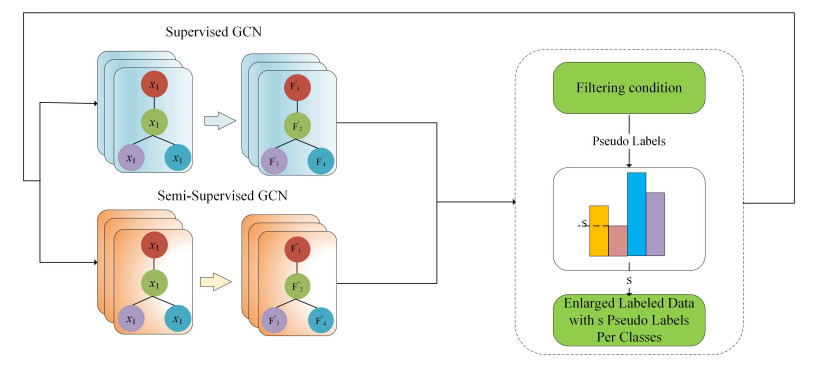
In the semi-supervised learning field, Graph Convolution Network (GCN), as a variant model of GNN, has achieved promising results for non-Euclidean data by introducing convolution into GNN. However, GCN and its variant models fail to safely use the information of risk unlabeled data, which will degrade the performance of semi-supervised learning. Therefore, we propose a Safe GCN framework (Safe-GCN) to improve the learning performance. In the Safe-GCN, we design an iterative process to label the unlabeled data. In each iteration, a GCN and its supervised version (S-GCN) are learned to find the unlabeled data with high confidence. The high-confidence unlabeled data and their pseudo labels are then added to the label set. Finally, both added unlabeled data and labeled ones are used to train a S-GCN which can achieve the safe exploration of the risk unlabeled data and enable safe use of large numbers of unlabeled data. The performance of Safe-GCN is evaluated on three well-known citation network datasets and the obtained results demonstrate the effectiveness of the proposed framework over several graph-based semi-supervised learning methods.

| [1] | L. Luo, K. Liu, D. Peng, Y. Ying, X. Zhang, A motif-based graph neural network to reciprocal recommendation for online dating, in International Conference on Neural Information Processing, Springer, (2020), 102–114. https://doi.org/10.1007/978-3-030-63833-7_9 |
| [2] | A. Fout, J. Byrd, B. Shariat, A. Ben-Hur, Protein interface prediction using graph convolutional networks, in Advances in Neural Information Processing Systems 30 (NIPS 2017), 30 (2017), 1–10. |
| [3] |
Y. B. Wang, Z. H. You, S. Yang, H. C. Yi, Z. H. Chen, K. Zheng, A deep learning-based method for drug-target interaction prediction based on long short-term memory neural network, BMC Med. Inf. Decis. Making, 20 (2020), 1–9. https://doi.org/10.1186/s12911-020-1052-0 doi: 10.1186/s12911-020-1052-0

|
| [4] |
X. M. Zhang, L. Liang, L. Liu, M. J. Tang, Graph neural networks and their current applications in bioinformatics, Front. Genet., 12 (2021), 690049. https://doi.org/10.3389/fgene.2021.690049 doi: 10.3389/fgene.2021.690049
|
| [5] |
J. Zhou, G. Cui, S. Hu, Z. Zhang, C. Yang, Z. Liu, et al., Graph neural networks: A review of methods and applications, AI Open, 1 (2020), 57–81. https://doi.org/10.1016/j.aiopen.2021.01.001 doi: 10.1016/j.aiopen.2021.01.001
|
| [6] | J. Bruna, W. Zaremba, A. Szlam, Y. LeCun, Spectral networks and locally connected networks on graphs, preprint, arXiv: 1312.6203. |
| [7] | M. Henaff, J. Bruna, Y. LeCun, Deep convolutional networks on graph-structured data, preprint, arXiv: 1506.05163. |
| [8] | J. Atwood, D. Towsley, Diffusion-convolutional neural networks, in Advances in Neural Information Processing Systems 29 (NIPS 2016), 29 (2016), 1–9. |
| [9] | T. N. Kipf, M. Welling, Semi-supervised classification with graph convolutional networks, preprint, arXiv: 1609.02907. |
| [10] | W. Hamilton, Z. Ying, J. Leskovec, Inductive representation learning on large graphs, in Advances in Neural Information Processing Systems 30 (NIPS 2017), 30 (2017), 1–11. |
| [11] | J. Chen, T. Ma, C. Xiao, Fastgcn: fast learning with graph convolutional networks via importance sampling, preprint, arXiv: 1801.10247. |
| [12] | F. Wu, A. Souza, T. Zhang, C. Fifty, T. Yu, K. Weinberger, Simplifying graph convolutional networks, in International Conference on Machine Learning, (2019), 6861–6871. |
| [13] | J. Du, S. Zhang, G. Wu, J. Moura, S. Kar, Topology adaptive graph convolutional networks, preprint, arXiv: 1710.10370. |
| [14] | P. Veličković, G. Cucurull, A. Casanova, A. Romero, P. Lio, Y. Bengio, Graph attention networks, preprint, arXiv: 1710.10903. |
| [15] | D. Kim, A. Oh, How to find your friendly neighborhood: Graph attention design with self-supervision, preprint, arXiv: 2204.04879. |
| [16] |
L. Zhu, H. Fan, Y. Luo, M. Xu, Y. Yang, Few-shot common-object reasoning using common-centric localization network, IEEE Trans. Image Process., 30 (2021), 4253–4262. https://doi.org/10.1109/TIP.2021.3070733 doi: 10.1109/TIP.2021.3070733
|
| [17] | W. Chiang, X. Liu, S. Si, Y. Li, S. Bengio, C. J. Hsieh, Cluster-gcn: An efficient algorithm for training deep and large graph convolutional networks, in Proceedings of the 25th ACM SIGKDD International Conference on Knowledge Discovery & Data Mining, (2019), 257–266. https://doi.org/10.1145/3292500.3330925 |
| [18] | H. Pei, B. Wei, K. C. C. Chang, Y. Lei, B. Yang, Geom-gcn: Geometric graph convolutional networks, preprint, arXiv: 2002.05287. |
| [19] |
B. Yu, Y. Lee, K. Sohn, Forecasting road traffic speeds by considering area-wide spatio-temporal dependencies based on a graph convolutional neural network, Transp. Res. Part C Emerging Technol., 114 (2020), 189–204. https://doi.org/10.1016/j.trc.2020.02.013 doi: 10.1016/j.trc.2020.02.013
|
| [20] |
O. Chapelle, B. Scholkopf, A. Zien, Semi-supervised learning [book reviews], IEEE Trans. Neural Networks, 20 (2009), 542. https://doi.org/10.1109/TNN.2009.2015974 doi: 10.1109/TNN.2009.2015974
|
| [21] | A. Singh, R. Nowak, J. Zhu, Unlabeled data: Now it helps, now it doesn't, in Advances in Neural Information Processing Systems 21 (NIPS 2008), 21 (2008), 1–8. |
| [22] |
N. V. Chawla, G. Karakoulas, Learning from labeled and unlabeled data: An empirical study across techniques and domains, J. Artif. Intell. Res., 23 (2005), 331–366. https://doi.org/10.1613/jair.1509 doi: 10.1613/jair.1509
|
| [23] | H. Gan, N. Sang, X. Chen, Semi-supervised kernel minimum squared error based on manifold structure, in International Symposium on Neural Networks, Springer, (2013), 265–272. https://doi.org/10.1007/978-3-642-39065-4_33 |
| [24] | Y. Wu, Y. Lin, X. Dong, Y. Yan, W. Ouyang, Y. Yang, Exploit the unknown gradually: One-shot video-based person re-identification by stepwise learning, in Proceedings of the IEEE Conference on Computer Vision and Pattern Recognition, (2018), 5177–5186. |
| [25] |
Y. Wu, Y. Lin, X. Dong, Y. Yan, W. Bian, Y. Yang, Progressive learning for person re-identification with one example, IEEE Trans. Image Process., 28 (2019), 2872–2881. https://doi.org/10.1109/TIP.2019.2891895 doi: 10.1109/TIP.2019.2891895
|
| [26] | Z. Hu, Z. Yang, X. Hu, R. Nevatia, Simple: similar pseudo label exploitation for semi-supervised classification, in Proceedings of the IEEE/CVF Conference on Computer Vision and Pattern Recognition, (2021), 15099–15108. |
| [27] | Q. Li, Z. Han, X. M. Wu, Deeper insights into graph convolutional networks for semi-supervised learning, in Thirty-Second AAAI conference on artificial intelligence, 2018. |
| [28] | K. Sun, Z. Lin, Z. Zhu, Multi-stage self-supervised learning for graph convolutional networks on graphs with few labeled nodes, in Proceedings of the AAAI Conference on Artificial Intelligence, 34 (2020), 5892–5899. https://doi.org/10.1609/aaai.v34i04.6048 |
| [29] | Z. Zhou, S. Zhang, Z. Huang, Dynamic self-training framework for graph convolutional networks, in International Conference on Learning Representations, 2019. |
| [30] |
D. C. G. Pedronette, L. J. Latecki, Rank-based self-training for graph convolutional networks, Inf. Process. Manage., 58 (2021), 102443. https://doi.org/10.1016/j.ipm.2020.102443 doi: 10.1016/j.ipm.2020.102443
|
| [31] |
H. Scudder, Probability of error of some adaptive pattern-recognition machines, IEEE Trans. Inf. Theory, 11 (1965), 363–371. https://doi.org/10.1109/TIT.1965.1053799 doi: 10.1109/TIT.1965.1053799
|
| [32] |
Y. Yang, Y. Zhuang, Y. Pan, Multiple knowledge representation for big data artificial intelligence: framework, applications, and case studies, Front. Inf. Technol. Electron. Eng., 22 (2021), 1551–1558. https://doi.org/10.1631/FITEE.2100463 doi: 10.1631/FITEE.2100463
|
| [33] |
P. Sen, G. Namata, M. Bilgic, L. Getoor, B. Galligher, T. Eliassi-Rad, Collective classification in network data, AI Mag., 29 (2008), 93. https://doi.org/10.1609/aimag.v29i3.2157 doi: 10.1609/aimag.v29i3.2157
|
| [34] | J. Klicpera, A. Bojchevski, S. Günnemann, Predict then propagate: Graph neural networks meet personalized pagerank, preprint, arXiv: 1810.05997. |
| [35] | K. K. Thekumparampil, C. Wang, S. Oh, L. J. Li, Attention-based graph neural network for semi-supervised learning, preprint, arXiv: 1803.03735. |
| [36] |
C. Cortes, V. Vapnik, Support-vector networks, Mach. Learn., 20 (1995), 273–297. https://doi.org/10.1007/BF00994018 doi: 10.1007/BF00994018
|
| [37] |
D. E. Rumelhart, G. E. Hinton, R. J. Williams, Learning representations by back-propagating errors, Nature, 323 (1986), 533–536. https://doi.org/10.1038/323533a0 doi: 10.1038/323533a0
|


Figures(4) / Tables(5)

Zhi Yang, Yadong Yan, Haitao Gan, Jing Zhao, Zhiwei Ye. A safe semi-supervised graph convolution network[J]. Mathematical Biosciences and Engineering, 2022, 19(12): 12677-12692. doi: 10.3934/mbe.2022592


 DownLoad: