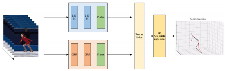
Body posture estimation has been a hot branch in the field of computer vision. This work focuses on one of its typical applications: recognition of various body postures in sports scenes. Existing technical methods were mostly established on the basis of convolution neural network (CNN) structures, due to their strong visual information sensing ability. However, sports scenes are highly dynamic, and many valuable contextual features can be extracted from multimedia frame sequences. To handle the current challenge, this paper proposes a hybrid neural network-based intelligent body posture estimation system for sports scenes. Specifically, a CNN unit and a long short-term memory (LSTM) unit are employed as the backbone network in order to extract key-point information and temporal information from video frames, respectively. Then, a semi-supervised learning-based computing framework is developed to output estimation results. It can make training procedures using limited labeled samples. Finally, through extensive experiments, it is proved that the proposed body posture estimation method in this paper can achieve proper estimation effect in real-world frame samples of sports scenes.
Citation: Liguo Zhang, Liangyu Zhao, Yongtao Yan. A hybrid neural network-based intelligent body posture estimation system in sports scenes[J]. Mathematical Biosciences and Engineering, 2024, 21(1): 1017-1037. doi: 10.3934/mbe.2024042
Body posture estimation has been a hot branch in the field of computer vision. This work focuses on one of its typical applications: recognition of various body postures in sports scenes. Existing technical methods were mostly established on the basis of convolution neural network (CNN) structures, due to their strong visual information sensing ability. However, sports scenes are highly dynamic, and many valuable contextual features can be extracted from multimedia frame sequences. To handle the current challenge, this paper proposes a hybrid neural network-based intelligent body posture estimation system for sports scenes. Specifically, a CNN unit and a long short-term memory (LSTM) unit are employed as the backbone network in order to extract key-point information and temporal information from video frames, respectively. Then, a semi-supervised learning-based computing framework is developed to output estimation results. It can make training procedures using limited labeled samples. Finally, through extensive experiments, it is proved that the proposed body posture estimation method in this paper can achieve proper estimation effect in real-world frame samples of sports scenes.

| [1] |
Y. Zon, G. Huang, A feature dimension reduction technology for predicting ddos intrusion behavior in multimedia internet of things, Multimedia Tools Appl., 80 (2021), 22671–22684. https://doi.org/10.1007/s11042-019-7591-7 doi: 10.1007/s11042-019-7591-7

|
| [2] |
T. Vijayakumar, R. Vinothkanna, M. Duraipandian, Fusion based feature extraction analysis of ecg signal interpretation–a systematic approach, J. Artif. Intell., 3 (2021), 1–16. https://doi.org/10.36548/jaicn.2021.1.001 doi: 10.36548/jaicn.2021.1.001
|
| [3] | X. Zhu, F. Ma, F. Ding, Z. Guo, J. Yang, K. Yu, A low-latency edge computation offloading scheme for trust evaluation in finance-level artificial intelligence of things, IEEE Internet Things J., 2023. https://doi.org/10.1109/JIOT.2023.3297834 |
| [4] |
D. Meng, Y. Xiao, Z. Guo, A. Jolfaei, L. Qin, X. Lu, et al., A data-driven intelligent planning model for uavs routing networks in mobile internet of things, Comput. Commun., 179 (2021), 231–241. https://doi.org/10.1016/j.comcom.2021.08.014 doi: 10.1016/j.comcom.2021.08.014
|
| [5] |
Y. Zhu, W. Lu, R. Zhang, R. Wang, D. Robbins, Dual-channel cascade pose estimation network trained on infrared thermal image and groundtruth annotation for real-time gait measurement, Med. Image Anal., 79 (2022), 102435. https://doi.org/10.1016/j.media.2022.102435 doi: 10.1016/j.media.2022.102435
|
| [6] |
S. K. Prabhakar, S. W. Lee, Holistic approaches to music genre classification using efficient transfer and deep learning techniques, Expert Syst. Appl., 211 (2023), 118636. https://doi.org/10.1016/j.eswa.2022.118636 doi: 10.1016/j.eswa.2022.118636
|
| [7] | Z. Guo, Q. Zhang, F. Ding, X. Zhu, K. Yu, A novel fake news detection model for context of mixed languages through multiscale transformer, IEEE Trans. Comput. Social Syst., 2023. https://doi.org/10.1109/TCSS.2023.3298480 |
| [8] |
M. P. van Dijk, M. Kok, M. A. Berger, M. J. Hoozemans, D. H. Veeger, Machine learning to improve orientation estimation in sports situations challenging for inertial sensor use, Front. Sports Active Living, 3 (2021), 670263. https://doi.org/10.3389/fspor.2021.670263 doi: 10.3389/fspor.2021.670263
|
| [9] |
S. Jang, J. Jang, Deep learning image processing technology for vehicle occupancy detection, J. Korea Inst. Inf. Commun. Eng., 25 (2021), 1026–1031. https://doi.org/10.6109/jkiice.2021.25.8.1026 doi: 10.6109/jkiice.2021.25.8.1026
|
| [10] |
I. Akhter, A. Jalal, K. Kim, Adaptive pose estimation for gait event detection using context-aware model and hierarchical optimization, J. Electr. Eng. Technol., 16 (2021), 2721–2729. https://doi.org/10.1007/s42835-021-00756-y doi: 10.1007/s42835-021-00756-y
|
| [11] |
J. Yang, L. Jia, Z. Guo, Y. Shen, X. Li, Z. Mou, et al., Prediction and control of water quality in recirculating aquaculture system based on hybrid neural network, Eng. Appl. Artif. Intell., 121 (2023), 106002. https://doi.org/10.1016/j.engappai.2023.106002 doi: 10.1016/j.engappai.2023.106002
|
| [12] |
P. Pareek, A. Thakkar, A survey on video-based human action recognition: recent updates, datasets, challenges, and applications, Artif. Intell. Rev., 54 (2021), 2259–2322. https://doi.org/10.1007/s10462-020-09904-8 doi: 10.1007/s10462-020-09904-8
|
| [13] |
L. H. Palucci Vieira, P. R. Santiago, A. Pinto, R. Aquino, R. d. S. Torres, F. A. Barbieri, Automatic markerless motion detector method against traditional digitisation for 3-dimensional movement kinematic analysis of ball kicking in soccer field context, Int. J. Environ. Res. Public Health, 19 (2022), 1179. https://doi.org/10.3390/ijerph19031179 doi: 10.3390/ijerph19031179
|
| [14] |
G. Lin, Y. Tang, X. Zou, C. Wang, Three-dimensional reconstruction of guava fruits and branches using instance segmentation and geometry analysis, Comput. Electron. Agric., 184 (2021), 106107. https://doi.org/10.1016/j.compag.2021.106107 doi: 10.1016/j.compag.2021.106107
|
| [15] | Z. Luo, R. Hachiuma, Y. Yuan, K. Kitani, Dynamics-regulated kinematic policy for egocentric pose estimation, Adv. Neural Inf. Process. Syst., 34 (2021), 25019–25032. |
| [16] |
C. Fang, T. Zhang, H. Zheng, J. Huang, K. Cuan, Pose estimation and behavior classification of broiler chickens based on deep neural networks, Comput. Electron. Agric., 180 (2021), 105863. https://doi.org/10.1016/j.compag.2020.105863 doi: 10.1016/j.compag.2020.105863
|
| [17] |
T. Huang, Q. Zhang, X. Tang, S. Zhao, X. Lu, A novel fault diagnosis method based on cnn and lstm and its application in fault diagnosis for complex systems, Artif. Intell. Rev., 55 (2022), 1289–1315. https://doi.org/10.1007/s10462-021-09993-z doi: 10.1007/s10462-021-09993-z
|
| [18] | B. Zhang, Y. Wang, W. Hou, H. Wu, J. Wang, M. Okumura, et al., Flexmatch: Boosting semi-supervised learning with curriculum pseudo labeling, Adv. Neural Inf. Process. Syst., 34 (2021), 18408–18419. |
| [19] |
Z. Guo, K. Yu, K. Konstantin, S. Mumtaz, W. Wei, P. Shi, et al., Deep collaborative intelligence-driven traffic forecasting in green internet of vehicles, IEEE Trans. Green Commun. Networking, 7 (2023), 1023–1035. https://doi.org/10.1109/TGCN.2022.3193849 doi: 10.1109/TGCN.2022.3193849
|
| [20] |
P. Jarvis, A. Turner, P. Read, C. Bishop, Reactive strength index and its associations with measures of physical and sports performance: A systematic review with meta-analysis, Sports Med., 52 (2022), 301–330. https://doi.org/10.1007/s40279-021-01566-y doi: 10.1007/s40279-021-01566-y
|
| [21] |
Ž. Kozinc, G. Marković, V. Hadžić, N. Šarabon, Relationship between force-velocity-power profiles and inter-limb asymmetries obtained during unilateral vertical jumping and singe-joint isokinetic tasks, J. Sports Sci., 39 (2021), 248–258. https://doi.org/10.1080/02640414.2020.1816271 doi: 10.1080/02640414.2020.1816271
|
| [22] |
L. K. Topham, W. Khan, D. Al-Jumeily, A. Hussain, Human body pose estimation for gait identification: A comprehensive survey of datasets and models, ACM Comput. Surv., 55 (2022), 1–42. https://doi.org/10.1145/3533384 doi: 10.1145/3533384
|
| [23] |
J. Yang, F. Lin, C. Chakraborty, K. Yu, Z. Guo, A. T. Nguyen, et al., A parallel intelligence-driven resource scheduling scheme for digital twins-based intelligent vehicular systems, IEEE Trans. Intell. Veh., 8 (2023), 2770–2785. https://doi.org/10.1109/TIV.2023.3237960 doi: 10.1109/TIV.2023.3237960
|
| [24] |
T. W. Dunn, J. D. Marshall, K. S. Severson, D. E. Aldarondo, D. G. Hildebrand, S. N. Chettih, et al., Geometric deep learning enables 3d kinematic profiling across species and environments, Nat. Methods, 18 (2021), 564–573. https://doi.org/10.1038/s41592-021-01106-6 doi: 10.1038/s41592-021-01106-6
|
| [25] |
Z. Guo, D. Meng, C. Chakraborty, X. R. Fan, A. Bhardwaj, K. Yu, Autonomous behavioral decision for vehicular agents based on cyber-physical social intelligence, IEEE Trans. Comput. Social Syst., 10 (2022), 2111–2122. https://doi.org/10.1109/TCSS.2022.3212864 doi: 10.1109/TCSS.2022.3212864
|
| [26] |
J. Huang, F. Yang, C. Chakraborty, Z. Guo, H. Zhang, L. Zhen, et al., Opportunistic capacity based resource allocation for 6g wireless systems with network slicing, Future Gener. Comput. Syst., 140 (2023), 390–401. https://doi.org/10.1016/j.future.2022.10.032 doi: 10.1016/j.future.2022.10.032
|
| [27] |
Q. Li, L. Liu, Z. Guo, P. Vijayakumar, F. Taghizadeh-Hesary, K. Yu, Smart assessment and forecasting framework for healthy development index in urban cities, Cities, 131 (2022), 103971. https://doi.org/10.1016/j.cities.2022.103971 doi: 10.1016/j.cities.2022.103971
|
| [28] | D. Ravishyam, D. Samiappan, Comparative study of machine learning with novel feature extraction and transfer learning to perform detection of glaucoma in fundus retinal images, in Soft Computing: Theories and Applications: Proceedings of SoCTA 2020, Volume 2, Springer, (2021), 419–429. |
| [29] | S. Wan, Y. Zhan, L. Liu, B. Yu, S. Pan, C. Gong, Contrastive graph poisson networks: Semi-supervised learning with extremely limited labels, Adv. Neural Inf. Process. Syst., 34 (2021), 6316–6327. |
| [30] |
Y. Chen, L. Liu, V. Phonevilay, K. Gu, R. Xia, J. Xie, et al., Image super-resolution reconstruction based on feature map attention mechanism, Appl. Intell., 51 (2021), 4367–4380. https://doi.org/10.1007/s10489-020-02116-1 doi: 10.1007/s10489-020-02116-1
|
| [31] |
O. Oladipo, E. O. Omidiora, V. C. Osamor, A novel genetic-artificial neural network based age estimation system, Sci. Rep., 12 (2022), 19290. https://doi.org/10.1038/s41598-022-23242-5 doi: 10.1038/s41598-022-23242-5
|
| [32] |
K. Gasmi, I. B. Ltaifa, G. Lejeune, H. Alshammari, L. B. Ammar, M. A. Mahmood, Optimal deep neural network-based model for answering visual medical question, Cybern. Syst., 53 (2022), 403–424. https://doi.org/10.1080/01969722.2021.2018543 doi: 10.1080/01969722.2021.2018543
|
| [33] |
Z. Guo, Y. Shen, A. K. Bashir, M. Imran, N. Kumar, D. Zhang, et al., Robust spammer detection using collaborative neural network in internet-of-things applications, IEEE Internet Things J., 8 (2021), 9549–9558, https://doi.org/10.1109/JIOT.2020.3003802 doi: 10.1109/JIOT.2020.3003802
|
| [34] |
B. Artacho, A. Savakis, Unipose+: A unified framework for 2d and 3d human pose estimation in images and videos, IEEE Trans. Pattern Anal. Mach. Intell., 44 (2021), 9641–9653. https://doi.org/10.1109/TPAMI.2021.3124736 doi: 10.1109/TPAMI.2021.3124736
|
| [35] |
Z. Guo, L. Tang, T. Guo, K. Yu, M. Alazab, A. Shalaginov, Deep graph neural network-based spammer detection under the perspective of heterogeneous cyberspace, Future Gener. Comput. Syst., 117 (2021), 205–218, https://doi.org/10.1016/j.future.2020.11.028 doi: 10.1016/j.future.2020.11.028
|
| [36] |
M. Yoo, Y. Na, H. Song, G. Kim, J. Yun, S. Kim, et al., Motion estimation and hand gesture recognition-based human-uav interaction approach in real time, Sensors, 22 (2022), 2513, https://doi.org/10.3390/s22072513 doi: 10.3390/s22072513
|
| [37] |
J. P. Sahoo, A. J. Prakash, P. Plawiak, S. Samantray, Real-time hand gesture recognition using fine-tuned convolutional neural network, Sensors, 22 (2022), 706, https://doi.org/10.3390/s22030706 doi: 10.3390/s22030706
|
| [38] | L. Mo, W. Liancheng, Design of sports competition aided evaluation system based on big data and motion recognition algorithm, ElectronicDesign Eng., 27 (2019), 6–10. |
| [39] |
J. Kim, S. Yang, B. Koo, S. Lee, S. Park, S. Kim, et al., semg-based hand posture recognition and visual feedback training for the forearm amputee, Sensors, 22 (2022), 7984, https://doi.org/10.3390/s22207984 doi: 10.3390/s22207984
|
| [40] |
J. Mu, S. Xian, J. Yu, J. Zhao, J. Song, Z. Li, et al., Synergistic enhancement properties of a flexible integrated pan/pvdf piezoelectric sensor for human posture recognition, Nanomaterials, 12 (2022), 1155. https://doi.org/10.3390/nano12071155 doi: 10.3390/nano12071155
|


Figures(10)

Liguo Zhang, Liangyu Zhao, Yongtao Yan. A hybrid neural network-based intelligent body posture estimation system in sports scenes[J]. Mathematical Biosciences and Engineering, 2024, 21(1): 1017-1037. doi: 10.3934/mbe.2024042


 DownLoad: