Characterization of spatiotemporal dynamics in EEG data during picture naming with optical flow patterns

V. Volpert; B. Xu; A. Tchechmedjiev; S. Harispe; A. Aksenov; Q. Mesnildrey; A. Beuter; V. Volpert; B. Xu; A. Tchechmedjiev; S. Harispe; A. Aksenov; Q. Mesnildrey; A. Beuter

doi:10.3934/mbe.2023507

Mathematical Biosciences and Engineering

2023, Volume 20, Issue 6: 11429-11463. doi: 10.3934/mbe.2023507

Previous Article Next Article

Research article Special Issues

Characterization of spatiotemporal dynamics in EEG data during picture naming with optical flow patterns

1.
Institut Camille Jordan, UMR 5208 CNRS, University Lyon 1, 69622 Villeurbanne, France
2.
EuroMov Digital Health in Motion, Univ Montpellier, IMT Mines Ales, Ales, France
3.
CorStim SAS, Montpellier, France

Academic Editor: Xiang-Sheng Wang

Received: 15 February 2023 Revised: 11 April 2023 Accepted: 17 April 2023 Published: 27 April 2023

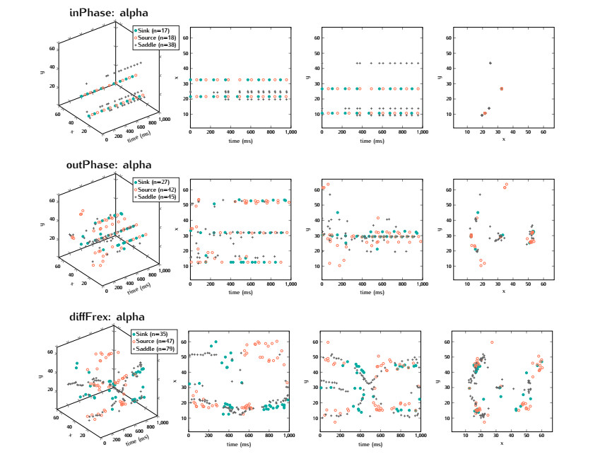
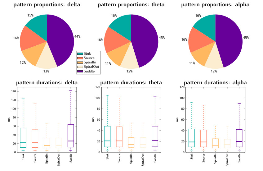
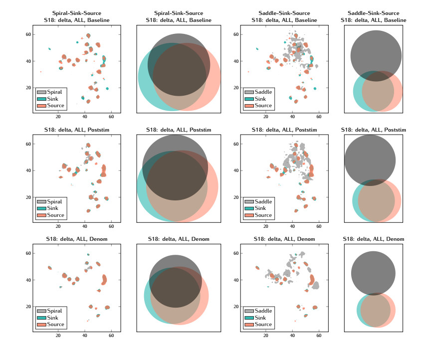
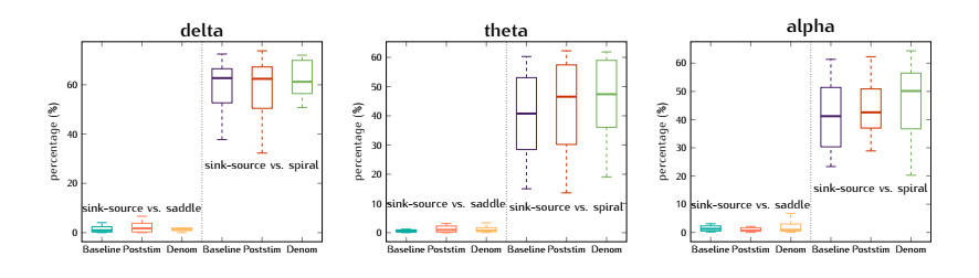
In this study, we investigate the spatiotemporal dynamics of the neural oscillations by analyzing the electric potential that arises from neural activity. We identify two types of dynamics based on the frequency and phase of oscillations: standing waves or as out-of-phase and modulated waves, which represent a combination of standing and moving waves. To characterize these dynamics, we use optical flow patterns such as sources, sinks, spirals and saddles. We compare analytical and numerical solutions with real EEG data acquired during a picture-naming task. Analytical approximation of standing waves helps us to establish some properties of pattern location and number. Specifically, sources and sinks are mainly located in the same location, while saddles are positioned between them. The number of saddles correlates with the sum of all the other patterns. These properties are confirmed in both the simulated and real EEG data. In particular, source and sink clusters in the EEG data overlap with each other with median percentages around 60%, and hence have high spatial correlation, while source/sink clusters overlap with saddle clusters in less than 1%, and have different locations. Our statistical analysis showed that saddles account for about 45% of all patterns, while the remaining patterns are present in similar proportions.
- human EEG data,
- spatiotemporal patterns,
- optical flow methods,
- picture-naming task
Citation: V. Volpert, B. Xu, A. Tchechmedjiev, S. Harispe, A. Aksenov, Q. Mesnildrey, A. Beuter. Characterization of spatiotemporal dynamics in EEG data during picture naming with optical flow patterns[J]. Mathematical Biosciences and Engineering, 2023, 20(6): 11429-11463. doi: 10.3934/mbe.2023507

Related Papers:

Abstract

In this study, we investigate the spatiotemporal dynamics of the neural oscillations by analyzing the electric potential that arises from neural activity. We identify two types of dynamics based on the frequency and phase of oscillations: standing waves or as out-of-phase and modulated waves, which represent a combination of standing and moving waves. To characterize these dynamics, we use optical flow patterns such as sources, sinks, spirals and saddles. We compare analytical and numerical solutions with real EEG data acquired during a picture-naming task. Analytical approximation of standing waves helps us to establish some properties of pattern location and number. Specifically, sources and sinks are mainly located in the same location, while saddles are positioned between them. The number of saddles correlates with the sum of all the other patterns. These properties are confirmed in both the simulated and real EEG data. In particular, source and sink clusters in the EEG data overlap with each other with median percentages around 60%, and hence have high spatial correlation, while source/sink clusters overlap with saddle clusters in less than 1%, and have different locations. Our statistical analysis showed that saddles account for about 45% of all patterns, while the remaining patterns are present in similar proportions.

References

[1]	E. D. Adrian, K. Yamagiwa, The origin of the berger rhythm, Brain, 58 (1935), 323–351. https://doi.org/10.1093/brain/58.3.323 doi: 10.1093/brain/58.3.323
[2]	S. Vakulenko, V. Volpert, Generalized travelling waves for perturbed monotone reaction-diffusion systems, Nonlinear Anal. Theory Methods Appl., 46 (2001), 757–776. https://doi.org/10.1016/S0362-546X(00)00130-9 doi: 10.1016/S0362-546X(00)00130-9
[3]	L. Muller, F. Chavane, J. Reynolds, T. J. Sejnowski, Cortical travelling waves: mechanisms and computational principles, Nat. Rev. Neurosci., 19 (2018), 255–268. https://doi.org/10.1038/nrn.2018.20 doi: 10.1038/nrn.2018.20
[4]	L. Meyer-Baese, H. Watters, S. Keilholz, Spatiotemporal patterns of spontaneous brain activity: a mini-review, Neurophotonics, 9 (2022), 1–17. https://doi.org/10.1117/1.NPh.9.3.032209 doi: 10.1117/1.NPh.9.3.032209
[5]	W. Klimesch, S. Hanslmayr, P. Sauseng, W. R. Gruber, M. Doppelmayr, P1 and traveling alpha waves: Evidence for evoked oscillations, J. Neurophysiol., 97 (2007), 1311–1318. PMID: 17167063. https://doi.org/10.1152/jn.00876.2006 doi: 10.1152/jn.00876.2006
[6]	T. M. Patten, C. J. Rennie, P. A. Robinson, P. Gong, Human cortical traveling waves: Dynamical properties and correlations with responses, PLoS One, 7 (2012), 1–10. https://doi.org/10.1371/journal.pone.0038392 doi: 10.1371/journal.pone.0038392
[7]	M. Massimini, R. Huber, F. Ferrarelli, S. Hill, G. Tononi, The sleep slow oscillation as a traveling wave, J. Neurosci., 24 (2004), 6862–6870. https://doi.org/10.1523/JNEUROSCI.1318-04.2004 doi: 10.1523/JNEUROSCI.1318-04.2004
[8]	A. Alamia, R. VanRullen, Alpha oscillations and traveling waves: Signatures of predictive coding, PLoS Biol., 17 (2019), 1–26. https://doi.org/10.1371/journal.pbio.3000487 doi: 10.1371/journal.pbio.3000487
[9]	T. Sato, I. Nauhaus, M. Carandini, Traveling waves in visual cortex, Neuron, 75 (2012), 218–229. https://doi.org/10.1016/j.neuron.2012.06.029 doi: 10.1016/j.neuron.2012.06.029
[10]	A. Benítez-Burraco, E. Murphy, Why brain oscillations are improving our understanding of language, Front. Behav. Neurosci., 13 (2019). https://doi.org/10.3389/fnbeh.2019.00190
[11]	A. Zauner, W. Gruber, N. A. Himmelstoß, J. Lechinger, W. Klimesch, Lexical access and evoked traveling alpha waves, NeuroImage, 91 (2014), 252–261. https://doi.org/10.1016/j.neuroimage.2014.01.041 doi: 10.1016/j.neuroimage.2014.01.041
[12]	D. M. Alexander, P. Jurica, C. Trengove, A. R. Nikolaev, S. Gepshtein, M. Zvyagintsev, et al., Traveling waves and trial averaging: The nature of single-trial and averaged brain responses in large-scale cortical signals, NeuroImage, 73 (2013), 95–112. https://doi.org/10.1016/j.neuroimage.2013.01.016 doi: 10.1016/j.neuroimage.2013.01.016
[13]	Y. Nir, R. Staba, T. Andrillon, V. Vyazovskiy, C. Cirelli, I. Fried, et al., Regional slow waves and spindles in human sleep, Neuron, 70 (2011), 153–169. https://doi.org/10.1016/j.neuron.2011.02.043 doi: 10.1016/j.neuron.2011.02.043
[14]	L. Muller, G. Piantoni, D. Koller, S. S. Cash, E. Halgren, T. J. Sejnowski, Rotating waves during human sleep spindles organize global patterns of activity that repeat precisely through the night, eLife, 5 (2016), e17267. https://doi.org/10.7554/eLife.17267 doi: 10.7554/eLife.17267
[15]	X. Huang, W. Xu, J. Liang, K. Takagaki, X. Gao, J.-Y. Wu, Spiral wave dynamics in neocortex, Neuron, 68 (2010), 978–990. https://doi.org/10.1016/j.neuron.2010.11.007 doi: 10.1016/j.neuron.2010.11.007
[16]	D. Lehmann, H. Ozaki, I. Pal, Eeg alpha map series: brain micro-states by space-oriented adaptive segmentation, Electroencephalogr. Clin. Neurophysiol., 67 (1987), 271–288. https://doi.org/10.1016/0013-4694(87)90025-3 doi: 10.1016/0013-4694(87)90025-3
[17]	T. Koenig, D. Lehmann, M. Merlo, K. Kochi, D. Hell, M. Koukkou, A deviant eeg brain microstate in acute, neuroleptic-naive schizophrenics at rest, Eur. Arch. Psychiatry Clin. Neurosci., 249 (1999), 205–211. https://doi.org/10.1007/s004060050088 doi: 10.1007/s004060050088
[18]	R. Grave de Peralta Menendez, M. M. Murray, C. M. Michel, R. Martuzzi, S. L. Gonzalez Andino, Electrical neuroimaging based on biophysical constraints, NeuroImage, 21 (2004), 527–539. https://doi.org/10.1016/j.neuroimage.2003.09.051 doi: 10.1016/j.neuroimage.2003.09.051
[19]	H. Yuan, V. Zotev, R. Phillips, W. C. Drevets, J. Bodurka, Spatiotemporal dynamics of the brain at rest - exploring eeg microstates as electrophysiological signatures of bold resting state networks, Neuroimage, 60 (2012), 2062–2072. https://doi.org/10.1016/j.neuroimage.2012.02.031 doi: 10.1016/j.neuroimage.2012.02.031
[20]	L. Brechet, D. Brunet, G. Birot, R. Gruetter, C. M. Michel, J. Jorge, Capturing the spatiotemporal dynamics of self-generated, task-initiated thoughts with eeg and fmri, Neuroimage, 194 (2019), 82–92. https://doi.org/10.1016/j.neuroimage.2019.03.029 doi: 10.1016/j.neuroimage.2019.03.029
[21]	M. Hassan, P. Benquet, A. Biraben, C. Berrou, O. Dufor, F. Wendling, Dynamic reorganization of functional brain networks during picture naming, Cortex, 73 (2015), 276–288. https://doi.org/10.1016/j.cortex.2015.08.019 doi: 10.1016/j.cortex.2015.08.019
[22]	A. Grappe, S. V. Sarma, P. Sacré, J. González-Martínez, C. Liégeois-Chauvel, F.-X. Alario, An intracerebral exploration of functional connectivity during word production, J. Comput. Neurosci., 46 (2019), 125–140. https://doi.org/10.1007/s10827-018-0699-3 doi: 10.1007/s10827-018-0699-3
[23]	G. Hartwigsen, A. Stockert, L. Charpentier, M. Wawrzyniak, J. Klingbeil, K. Wrede, et al., Short-term modulation of the lesioned language network, eLife, 9 (2020), e54277. https://doi.org/10.7554/eLife.54277 doi: 10.7554/eLife.54277
[24]	M. Laganaro, G. Python, U. Toepel, Dynamics of phonological–phonetic encoding in word production: Evidence from diverging erps between stroke patients and controls, Brain Lang., 126 (2013), 123–132. https://doi.org/10.1016/j.bandl.2013.03.004 doi: 10.1016/j.bandl.2013.03.004
[25]	A. Mheich, O. Dufor, S. Yassine, A. Kabbara, A. Biraben, F. Wendling, et al., Hd-eeg for tracking sub-second brain dynamics during cognitive tasks, Sci. Data, 8 (2021). https://doi.org/10.1038/s41597-021-00821-1
[26]	L. S. Hooi, H. Nisar, Y. V. Voon, Tracking of eeg activity using topographic maps, in 2015 IEEE International Conference on Signal and Image Processing Applications (ICSIPA), (2015), 287–291. https://doi.org/10.1109/ICSIPA.2015.7412206
[27]	R. G. Townsend, S. S. Solomon, S. C. Chen, A. N. Pietersen, P. R. Martin, S. G. Solomon, et al., Emergence of complex wave patterns in primate cerebral cortex, J. Neurosci., 35 (2015), 4657–4662. https://doi.org/10.1523/JNEUROSCI.4509-14.2015 doi: 10.1523/JNEUROSCI.4509-14.2015
[28]	R. G. Townsend, P. Gong, Detection and analysis of spatiotemporal patterns in brain activity, PLoS Comput. Biol., 14 (2018), 1–29. https://doi.org/10.1371/journal.pcbi.1006643 doi: 10.1371/journal.pcbi.1006643
[29]	Y. Liang, C. Song, M. Liu, P. Gong, C. Zhou, T. Knöpfel, Cortex-wide dynamics of intrinsic electrical activities: propagating waves and their interactions, J. Neurosci., 41 (2021), 3665–3678. https://doi.org/10.1523/JNEUROSCI.0623-20.2021 doi: 10.1523/JNEUROSCI.0623-20.2021
[30]	L. Muller, A. Reynaud, F. Chavane, A. Destexhe, The stimulus-evoked population response in visual cortex of awake monkey is a propagating wave, Nature Communications, 5 (2014), 3675. https://doi.org/10.1038/ncomms4675 doi: 10.1038/ncomms4675
[31]	G. B. Saturnino, O. Puonti, J. D. Nielsen, D. Antonenko, K. H. Madsen, A. Thielscher, Simnibs 2.1: A comprehensive pipeline for individualized electric field modelling for transcranial brain stimulation, bioRxiv, 2018.
[32]	G. B. Saturnino, H. R. Siebner, A. Thielscher, K. H. Madsen, Accessibility of cortical regions to focal tes: Dependence on spatial position, safety, and practical constraints, NeuroImage, 203 (2019), 116183. https://doi.org/10.1016/j.neuroimage.2019.116183 doi: 10.1016/j.neuroimage.2019.116183
[33]	J. Wackermann, D. Lehmann, C. Michel, W. Strik, Adaptive segmentation of spontaneous eeg map series into spatially defined microstates, Int. J. Psychophysiol., 14 (1993), 269–283. https://doi.org/10.1016/0166-1280(93)87137-3 doi: 10.1016/0166-1280(93)87137-3
[34]	G. Buzsaki, C. A. Anastassiou, C. Koch, The origin of extracellular fields and currents – EEG, ecog, lfp and spikes, Nat. Rev. Neurosci., 13 (2012), 407–420. https://doi.org/10.1038/nrn3241 doi: 10.1038/nrn3241
[35]	G. B. Saturnino, K. H. Madsen, H. R. Siebner, A. Thielscher, How to target inter-regional phase synchronization with dual-site transcranial alternating current stimulation, NeuroImage, 163 (2017), 68–80. https://doi.org/10.1016/j.neuroimage.2017.09.024 doi: 10.1016/j.neuroimage.2017.09.024
[36]	J. Eggermont, Brain Oscillations, Synchrony and Plasticity: Basic Principles and Application to Auditory-Related Disorders, Elsevier Science, 2021. https://doi.org/10.1016/C2019-0-00734-0
[37]	R. Oldfield, The assessment and analysis of handedness: The edinburgh inventory, Neuropsychologia, 9 (1971), 97–113. https://doi.org/10.1016/0028-3932(71)90067-4 doi: 10.1016/0028-3932(71)90067-4
[38]	J. G. Snodgrass, M. Vanderwart, A standardized set of 260 pictures: Norms for name agreement, image agreement, familiarity, and visual complexity, Journal of Experimental Psychology: Human Learning and Memory, 6 (1980), 174–215. https://doi.org/10.1037/0278-7393.6.2.174 doi: 10.1037/0278-7393.6.2.174
[39]	D. T. Sandwell, Biharmonic spline interpolation of geos-3 and seasat altimeter data, Geophysical Research Letters, 14 (1987), 139–142. https://doi.org/10.1029/GL014i002p00139 doi: 10.1029/GL014i002p00139
[40]	L. Marple, Computing the discrete-time "analytic" signal via FFT, IEEE Trans. Signal Process., 47 (1999), 2600–2603. https://doi.org/10.1109/78.782222 doi: 10.1109/78.782222
[41]	T. C. Ferree, Spline interpolation of the scalp eeg, Electrical Geodesics, Inc., 2000. Available from: https://www.researchgate.net/publication/265238579.
[42]	B. K. Horn, B. G. Schunck, Determining optical flow, Artif. Intell., 17 (1981), 185–203. https://doi.org/10.1016/0004-3702(81)90024-2
[43]	A. Thielscher, A. Antunes, G. B. Saturnino, Field modeling for transcranial magnetic stimulation: A useful tool to understand the physiological effects of TMS, in 2015 37th Annual International Conference of the IEEE Engineering in Medicine and Biology Society (EMBC), (2015), 222–225. https://doi.org/10.1109/EMBC.2015.7318340
[44]	Simnibs example dataset, 2022. Available from: https://simnibs.github.io/simnibs/build/html/dataset.html.
[45]	Neuroelectrics wiki, 2022. Available from: https://www.neuroelectrics.com/wiki/index.php/Neuroelectrics_Frequently_Asked_Questions_(FAQs)#What_do_I_need_to_consider_when_creating_a_stimulation_protocol.3F.

Reader Comments

Your name:*

Email:*
© 2023 the Author(s), licensee AIMS Press. This is an open access article distributed under the terms of the Creative Commons Attribution License (http://creativecommons.org/licenses/by/4.0)