Study on knowledge cooperation of interdisciplinary research team based on evolutionary game theory

Huan Zhao; Xi Chen; Huan Zhao; Xi Chen

doi:10.3934/mbe.2023386

Mathematical Biosciences and Engineering

2023, Volume 20, Issue 5: 8782-8799. doi: 10.3934/mbe.2023386

Previous Article Next Article

Research article Special Issues

Study on knowledge cooperation of interdisciplinary research team based on evolutionary game theory

Huan Zhao ^{1
,
,},
Xi Chen ²

1.
School of Management and Engineering, Capital University of Economics and Business, Beijing 10070, China
2.
Information Center, Capital University of Economics and Business, Beijing 10070, China

Academic Editor: Peng-Yeng Yin

Received: 08 December 2022 Revised: 20 January 2023 Accepted: 19 February 2023 Published: 07 March 2023

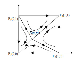
Based on knowledge sharing, a new kind of scientific research is up and coming in university interdisciplinary research teams via the current environment of organizational models. The success, however, depends on the knowledge inventory, the creative ability of the team members and their future insights. An attempt is made in this study to conceptualize a framework of an interdisciplinary research team based on game theory to analyze the dynamic propagation process of knowledge-sharing. Through simulation verification, a multi-symmetry evolution game model was built to analyze the impact of a member in selecting a decision-making strategy for the other member. The analysis reveals that the knowledge-sharing depends on mutual cooperation and trust between the researchers. Finally, reasonable suggestions are proposed in solving the problems in the process of building and developing the university interdisciplinary research team.

Keywords:

Citation: Huan Zhao, Xi Chen. Study on knowledge cooperation of interdisciplinary research team based on evolutionary game theory[J]. Mathematical Biosciences and Engineering, 2023, 20(5): 8782-8799. doi: 10.3934/mbe.2023386

Related Papers:

[1]	Yuriĭ G. Nikonorov, Irina A. Zubareva . On the behavior of geodesics of left-invariant sub-Riemannian metrics on the group $\operatorname{Aff}_{0}(\mathbb{R}) \times \operatorname{Aff}_{0}(\mathbb{R})$ . Electronic Research Archive, 2025, 33(1): 181-209. doi: 10.3934/era.2025010
[2]	Lakehal Belarbi . Ricci solitons of the $\mathbb{H}^{2} \times \mathbb{R}$ Lie group. Electronic Research Archive, 2020, 28(1): 157-163. doi: 10.3934/era.2020010
[3]	Margarida Camarinha . A natural 4th-order generalization of the geodesic problem. Electronic Research Archive, 2024, 32(5): 3396-3412. doi: 10.3934/era.2024157
[4]	Wen Teng, Xiansheng Dai . Nonabelian embedding tensors on 3-Lie algebras and 3-Leibniz-Lie algebras. Electronic Research Archive, 2025, 33(3): 1367-1383. doi: 10.3934/era.2025063
[5]	Shanshan Liu, Abdenacer Makhlouf, Lina Song . The full cohomology, abelian extensions and formal deformations of Hom-pre-Lie algebras. Electronic Research Archive, 2022, 30(8): 2748-2773. doi: 10.3934/era.2022141
[6]	Hongliang Chang, Yin Chen, Runxuan Zhang . A generalization on derivations of Lie algebras. Electronic Research Archive, 2021, 29(3): 2457-2473. doi: 10.3934/era.2020124
[7]	Yizheng Li, Dingguo Wang . Lie algebras with differential operators of any weights. Electronic Research Archive, 2023, 31(3): 1195-1211. doi: 10.3934/era.2023061
[8]	Kailash C. Misra, Sutida Patlertsin, Suchada Pongprasert, Thitarie Rungratgasame . On derivations of Leibniz algebras. Electronic Research Archive, 2024, 32(7): 4715-4722. doi: 10.3934/era.2024214
[9]	Pengliang Xu, Xiaomin Tang . Graded post-Lie algebra structures and homogeneous Rota-Baxter operators on the Schrödinger-Virasoro algebra. Electronic Research Archive, 2021, 29(4): 2771-2789. doi: 10.3934/era.2021013
[10]	Shaban Khidr, Salomon Sambou . $L^p$ -theory for the ${\partial }\overline{\partial}$ -equation and isomorphisms results. Electronic Research Archive, 2025, 33(1): 68-86. doi: 10.3934/era.2025004

Abstract

1. Introduction

Einstein metrics are pivotal in numerous domains of mathematical physics and differential geometry. They are also of interest in pure mathematics, particularly in the fields of geometric analysis and algebraic geometry. An Einstein metric can be regarded as a fixed solution (up to diffeomorphism and scaling) of the Hamilton Ricci flow equation. On a Riemannian manifold $(M, g)$ , a Ricci soliton is said to exist when there is a smooth vector field $X$ and a constant $\lambda$ in the reals that satisfy the condition stated below:

$\begin{equation*} R_{ij}+\frac{1}{2}(\mathcal{L}_{X}g)_{ij} = \lambda g_{ij}, \end{equation*}$

where $R_{ij}$ is the Ricci curvature tensor, and $\mathcal{L}_{X}g$ stands for the Lie derivative of $g$ with respect to the vector field $X$ . This concept was introduced by Hamilton in ^[1], and later utilized by Perelman in his proof of the long-standing Poincare conjecture ^[2]. Lauret further generalized the notion of Einstein metrics to algebraic Ricci solitons in the Riemannian context, introducing them as a natural extension in ^[3]. Subsequently, Onda and Batat applied this framework to pseudo-Riemannian Lie groups, achieving a complete classification of algebraic Ricci solitons in three-dimensional Lorentzian Lie groups in ^[4]. Additionally, they proved that within the framework of pseudo-Riemannian manifolds, there is algebraic Ricci solitons that are not of the conventional Ricci soliton type.

In ^[5], Etayo and Santamaria explored the concept of distinguished connections on $(J^{2} = \pm1)$ -metric manifolds. This sparked interest among mathematicians in studying Ricci solitons linked to various affine connections, which can be found in ^[6,7,8]. The Bott connection was introduced in earlier works (see^[9,10,11]). In ^[12], the authors developed a theory on geodesic variations under metric changes in a geodesic foliation, with the Bott connection serving as the primary natural connection respecting the foliation's structure. In ^[13], Wu and Wang studied affine Ricci solitons and quasi-statistical structures on three-dimensional Lorentzian Lie groups associated with the Bott connection. Furthermore, in ^[14,15], the authors examined the algebraic schouten solitons and affine Ricci solitons concerning various affine connections.

Inspired by Lauret's work, Wears introduced algebraic T-solitons, linking them to T-solitons in ^[16]. Later, in ^[7], Azami introduced Schouten solitons, as a new type of generalized Ricci soliton. In this paper, I focus on algebraic Schouten solitons concerning the Bott connection with three distributions, aiming to classify and describe them on three-dimensional Lorentzian Lie groups.

In Section 2, I introduce the fundamental notions associated with three-dimensional Lie groups and algebraic Schouten soliton. In Sections 3–5, I discuss and present algebraic Schouten solitons concerning the Bott connection on three-dimensional Lorentzian Lie groups, each focusing on a different type of distribution.

2. Preliminaries

In ^[17], Milnor conducted a survey of both classical and recent findings on left-invariant Riemannian metrics on Lie groups, particularly on three-dimensional unimodular Lie groups. Furthermore, in ^[18], Rahmani classified three-dimensional unimodular Lie groups in the Lorentzian context. The non-unimodular cases were handled in ^[19,20]. Throughout this paper, I use $\{G_{i}\}_{i = 1}^{7}$ for connected, simply connected three-dimensional Lie groups equipped with a left-invariant Lorentzian metric $g$ . Their corresponding Lie algebras are denoted by $\{\mathfrak{g_{i}}\}_{i = 1}^{7}$ , and each possess a pseudo-orthonormal basis $\{e_{1}, e_{2}, e_{3}\}$ (with $e_{3}$ timelike, see ^[4]). Let $\nabla^{LC}$ and $R^{LC}$ denote the Levi-Civita connection and curvature tensor of $G_{i}$ , respectively, then

$\begin{equation*} R^{LC}(X,Y)Z = \nabla^{LC}_{X}\nabla^{LC}_{Y}Z-\nabla^{LC}_{Y}\nabla^{LC}_{X}Z-\nabla^{LC}_{[X,Y]}Z. \end{equation*}$

The Ricci tensor of $(G_{i}, g)$ is defined as follows:

$\begin{equation*} \rho^{LC}(X,Y) = -g(R^{LC}(X,e_{1})Y,e_{1})-g(R^{LC}(X,e_{2})Y,e_{2})+g(R^{LC}(X,e_{3})Y,e_{3}). \end{equation*}$

Moreover, I have the expression for the Ricci operator $Ric^{LC}$ :

$\begin{equation*} \rho^{LC}(X,Y) = g(Ric^{LC}(X),Y). \end{equation*}$

Next, recall the Bott connection, denoted by $\nabla^{B}$ . Consider a smooth manifold $(M, g)$ that is equipped with the Levi-Civita connection $\nabla$ , and let $TM$ represent its tangent bundle, spanned by $\{e_{1}, e_{2}, e_{3}\}$ . I introduce a distribution $D$ spanned by $\{e_{1}, e_{2}\}$ and its orthogonal complement $D^{\perp}$ , which is spanned by $\{e_{3}\}$ . The Bott connection $\nabla^{B}$ associated with distribution $D$ is then defined as follows:

$\begin{equation} \nabla_{X}^{B}Y = \left\{ \begin{aligned} &\pi_{D}(\nabla^{LC}_{X}Y),\quad X,Y\in\Gamma^{\infty}(D),\\ &\pi_{D}([X,Y]),\quad X\in\Gamma^{\infty}(D^{\perp}),\; Y\in\Gamma^{\infty}(D),\\ &\pi_{D^{\perp}}([X,Y]),\quad X\in\Gamma^{\infty}(D),\; Y\in\Gamma^{\infty}(D^{\perp}),\\ &\pi_{D^{\perp}}(\nabla^{LC}_{X}Y),\quad X,Y\in\Gamma^{\infty}(D^{\perp}), \end{aligned} \right. \end{equation}$

(2.1)

where $\pi_{D}$ (respectively, $\pi_{D^{\perp}}$ ) denotes the projection onto $D$ (respectively, $D^{\perp}$ ). For a more detailed discussion, refer to ^[9,10,11,21]. I denote the curvature tensor of the Bott connection $\nabla^{B}$ by $R^{B}$ , which is defined as follows:

$\begin{equation} R^{B}(X,Y)Z = \nabla^{B}_{X}\nabla^{B}_{Y}Z-\nabla^{B}_{Y}\nabla^{B}_{X}Z-\nabla^{B}_{[X,Y]}Z. \end{equation}$

(2.2)

The Ricci tensor $\rho^{B}$ associated to the connection $\nabla^{B}$ is defined as:

$\begin{equation*} \rho^{B}(X,Y) = \frac{B(X,Y)+B(Y,X)}{2}, \end{equation*}$

where

$\begin{equation*} B(X,Y) = -g(R^{B}(X,e_{1})Y,e_{1})-g(R^{B}(X,e_{2})Y,e_{2})+g(R^{B}(X,e_{3})Y,e_{3}). \end{equation*}$

Using the Ricci tensor $\rho^{B}$ , the Ricci operator $Ric^{B}$ is given by:

$\begin{equation} \rho^{B}(X,Y) = g(Ric^{B}(X),Y). \end{equation}$

(2.3)

Then, I have the definition of the Schouten tensor as follows:

$\begin{equation*} S^{B}(e_{i},e_{j}) = \rho^{B}(e_{i},e_{j})-\frac{s^{B}}{4}g(e_{i},e_{j}), \end{equation*}$

where $s^{B}$ represents the scalar curvature. Moreover, I generalized the Schouten tensor to:

$\begin{equation*} S^{B}(e_{i},e_{j}) = \rho^{B}(e_{i},e_{j})-s^{B}\lambda_{0}g(e_{i},e_{j}), \end{equation*}$

where $\lambda_{0}$ is a real number. By ^[22], I obtain the expression of $s^{B}$ as

$\begin{equation*} s^{B} = \rho^{B}(e_{1},e_{1})+\rho^{B}(e_{2},e_{2})-\rho^{B}(e_{3},e_{3}). \end{equation*}$

Definition 1. A manifold $(G_{i}, g)$ is called an algebraic Schouten soliton with associated to the connection $\nabla^{B}$ if it satisfies:

$\begin{equation*} Ric^{B} = (s^{B}\lambda_{0}+c)Id+D^{B}, \end{equation*}$

where $c$ is a constant, and $D^{B}$ is a derivation of $\mathfrak{g}_{i}$ , i.e.,

$\begin{equation} D^{B}[X_{1},X_{2}] = [D^{B}X_{1},X_{2}]+[X_{1},D^{B}X_{2}],\quad for\; X_{1},X_{2}\in \mathfrak{g}_{i}. \end{equation}$

(2.4)

3. Algebraic Schouten soliton concerning connection $\nabla^{B}$

In this section, I derive the algebraic criterion for the three-dimensional Lorentzian Lie group to exhibit an algebraic Schouten soliton related to the connection $\nabla^{B}$ . Moreover, I indicate that $G_{4}$ and $G_{7}$ do not have such solitons.

3.1. Algebraic Schouten soliton of $G_{1}$

According to ^[4], I have the expression for $\mathfrak{g}_{1}$ :

$\begin{equation*} [e_{1},e_{2}] = \alpha e_{1}-\beta e_{3},\quad [e_{1},e_{3}] = -\alpha e_{1}-\beta e_{2},\quad [e_{2},e_{3}] = \beta e_{1}+\alpha e_{2}+\alpha e_{3}, \end{equation*}$

where $\alpha\neq0$ . From this, I derive the following theorem.

Theorem 2. If $(G_{1}, g)$ constitutes an algebraic Schouten soliton concerning connection $\nabla^{B}$ ; then, it fulfills the conditions: $\beta = 0$ and $c = -\frac{1}{2}\alpha^{2}+2(\alpha^{2}+\beta^{2})\lambda_{0}$ .

Proof. From ^[23], the expression for $Ric^{B}$ is as follows:

$\begin{equation*} Ric^{B}\left( \begin{matrix} e_{1}\\ e_{2}\\ e_{3} \end{matrix}\right) = \left( \begin{matrix} -(\alpha^{2}+\beta^{2}) & \alpha\beta & \frac{1}{2}\alpha\beta\\ \alpha\beta & -(\alpha^{2}+\beta^{2}) & -\frac{1}{2}\alpha^{2}\\ -\frac{1}{2}\alpha\beta & \frac{1}{2}\alpha^{2} & 0 \end{matrix} \right) \left( \begin{matrix} e_{1}\\ e_{2}\\ e_{3} \end{matrix}\right). \end{equation*}$

The scalar curvature is $s^{B} = -2(\alpha^{2}+\beta^{2})$ . Now, I can express $D^{B}$ as follows:

$\begin{equation*} \left\{ \begin{aligned} &D^{B}e_{1} = -(\alpha^{2}+\beta^{2}+s\lambda_{0}+c)e_{1}+\alpha\beta e_{2}+\frac{\alpha\beta}{2}e_{3},\\ &D^{B}e_{2} = \alpha\beta e_{1}-(\alpha^{2}+\beta^{2}+s\lambda_{0}+c)e_{2}-\frac{\alpha^{2}}{2}e_{3},\\ &D^{B}e_{3} = -\frac{\alpha\beta}{2}e_{1}+\frac{\alpha^{2}}{2}e_{2}+(2(\alpha^{2}+\beta^{2})\lambda_{0}-c)e_{3}. \end{aligned} \right. \end{equation*}$

Therefore, based on Eq (2.4), there is an algebraic Schouten soliton associated with $\nabla^{B}$ on $(G_{1}, g)$ , if and only if the following condition satisfies:

$\begin{equation*} \left\{ \begin{aligned} &\frac{5}{2}\alpha^{2}\beta+2\beta^{3}-2\lambda_{0}\beta(\alpha^{2}+\beta^{2})+c\beta = 0,\\ &\frac{\alpha^{3}}{2}+2\alpha\beta^{2}-2\lambda_{0}\alpha(\alpha^{2}+\beta^{2})+c\alpha = 0,\\ &\alpha^{2}\beta = 0,\\ &2\alpha^{2}\beta+\beta^{3}-4\lambda_{0}\beta(\alpha^{2}+\beta^{2})+2c\beta = 0,\\ &\frac{\alpha^{3}}{2}+\frac{3}{2}\alpha\beta^{2}-2\lambda_{0}\alpha(\alpha^{2}+\beta^{2})+c\alpha = 0. \end{aligned} \right. \end{equation*}$

Since $\alpha\neq0$ , I have $\beta = 0$ and $c = -\frac{1}{2}\alpha^{2}+2(\alpha^{2}+\beta^{2})\lambda_{0}$ . □

3.2. Algebraic Schouten soliton of $G_{2}$

According to ^[4], I have the expression for $\mathfrak{g}_{2}$ :

$\begin{equation*} [e_{1},e_{2}] = \gamma e_{2}-\beta e_{3},\quad [e_{1},e_{3}] = -\beta e_{2}-\gamma e_{3},\quad [e_{2},e_{3}] = \alpha e_{1}, \end{equation*}$

where $\gamma\neq0$ . From this, I derive the following theorem.

Theorem 3. If $(G_{2}, g)$ constitutes an algebraic Schouten soliton concerning the connection $\nabla^{B}$ , then it fulfills the conditions: $\alpha = 0$ and $c = -\beta^{2}-\gamma^{2}+(\beta^{2}+2\gamma^{2})\lambda_{0}$ .

Proof. From ^[23], the expression for $Ric^{B}$ is as follows:

$\begin{equation*} Ric^{B}\left( \begin{matrix} e_{1}\\ e_{2}\\ e_{3} \end{matrix}\right) = \left( \begin{matrix} -(\beta^{2}+\gamma^{2}) & 0 & 0\\ 0 & -(\gamma^{2}+\alpha\beta) & \frac{\alpha\gamma}{2}\\ 0 & -\frac{\alpha\gamma}{2} & 0 \end{matrix} \right) \left( \begin{matrix} e_{1}\\ e_{2}\\ e_{3} \end{matrix}\right). \end{equation*}$

The scalar curvature is $s^{B} = -(\beta^{2}+2\gamma^{2}+\alpha\beta)$ . Now, I can express $D^{B}$ as follows:

$\begin{equation*} \left\{ \begin{aligned} &D^{B}e_{1} = -(\beta^{2}+\gamma^{2}-(\beta^{2}+2\gamma^{2}+\alpha\beta)\lambda_{0}+c)e_{1},\\ &D^{B}e_{2} = -(\gamma^{2}+\alpha\beta-(\beta^{2}+2\gamma^{2}+\alpha\beta)\lambda_{0}+c)e_{2}+\frac{\alpha\gamma}{2}e_{3},\\ &D^{B}e_{3} = -\frac{\alpha\gamma}{2}e_{2}+((\beta^{2}+2\gamma^{2}+\alpha\beta)\lambda_{0}-c)e_{3}. \end{aligned} \right. \end{equation*}$

Therefore, based on Eq (2.4), there is an algebraic Schouten soliton associated with $\nabla^{B}$ on $(G_{2}, g)$ , if and only if the following condition satisfies:

$\begin{equation*} \left\{ \begin{aligned} &\alpha\gamma^{2}-\beta^{3}+\alpha\beta^{2}+(\beta^{2}+2\gamma^{2}+\alpha\beta)\beta\lambda_{0}-c\beta = 0,\\ &\gamma(\beta^{2}+\gamma^{2}+\alpha\beta-(\beta^{2}+2\gamma^{2}+\alpha\beta)\lambda_{0}+c) = 0,\\ &\alpha\gamma^{2}-\beta^{3}-2\beta\gamma^{2}-\alpha\beta^{2}+(\beta^{2}+2\gamma^{2}+\alpha\beta)\beta\lambda_{0}-c\beta = 0,\\ &\alpha(-\beta^{2}+\alpha\beta-(\beta^{2}+2\gamma^{2}+\alpha\beta)\lambda_{0}+c) = 0. \end{aligned} \right. \end{equation*}$

Suppose that $\alpha = 0$ , then $c = -\beta^{2}-\gamma^{2}+(\beta^{2}+2\gamma^{2})\lambda_{0}$ . If $\alpha\neq0$ , I have

$\begin{equation*} \left\{ \begin{aligned} &\beta(\beta^{2}+\gamma^{2}-(\beta^{2}+2\gamma^{2}+\alpha\beta)\lambda_{0}+c) = 0,\\ &\beta^{2}+\gamma^{2}+\alpha\beta-(\beta^{2}+2\gamma^{2}+\alpha\beta)\lambda_{0}+c = 0,\\ &-\beta^{2}+\alpha\beta-(\beta^{2}+2\gamma^{2}+\alpha\beta)\lambda_{0}+c = 0. \end{aligned} \right. \end{equation*}$

Since $\gamma\neq0$ , solving the equations of the above system gives $2\beta^{2}+\gamma^{2} = 0$ , which is a contradiction. □

3.3. Algebraic Schouten soliton of $G_{3}$

According to ^[4], I have the expression for $\mathfrak{g}_{3}$ :

$\begin{equation*} [e_{1},e_{2}] = -\gamma e_{3},\quad [e_{1},e_{3}] = -\beta e_{2},\quad [e_{2},e_{3}] = \alpha e_{1}. \end{equation*}$

From this, I derive the following theorem.

Theorem 4. If $(G_{3}, g)$ is an algebraic Schouten soliton concerning connection $\nabla^{B}$ ; then, one of the following cases holds:

i. $\alpha = \beta = \gamma = 0$ , for all $c$ ;

ii. $\alpha\neq0$ , $\beta = \gamma = 0$ , $c = 0$ ;

iii. $\alpha = \gamma = 0$ , $\beta\neq0$ , $c = 0$ ;

iv. $\alpha\neq0$ , $\beta\neq0$ , $\gamma = 0$ , $c = 0$ ;

v. $\alpha = \beta = 0$ , $\gamma\neq0$ , $c = 0$ ;

vi. $\alpha\neq0$ , $\beta = 0$ , $\gamma\neq0$ , $c = -\alpha\gamma+\alpha\gamma\lambda_{0}$ ;

vii. $\alpha = 0$ , $\beta\neq0$ , $\gamma\neq0$ , $c = -\beta\gamma+\beta\gamma\lambda_{0}$ .

Proof. From ^[23], the expression for $Ric^{B}$ is as follows:

$\begin{equation*} Ric^{B}\left( \begin{matrix} e_{1}\\ e_{2}\\ e_{3} \end{matrix}\right) = \left( \begin{matrix} -\beta\gamma & 0 & 0\\ 0 & -\alpha\gamma & 0\\ 0 & 0 & 0 \end{matrix} \right) \left( \begin{matrix} e_{1}\\ e_{2}\\ e_{3} \end{matrix}\right). \end{equation*}$

The scalar curvature is $s^{B} = -\gamma(\alpha+\beta)$ . Now, I can express $D^{B}$ as follows:

$\begin{equation*} \left\{ \begin{aligned} &D^{B}e_{1} = -(\beta\gamma-\gamma(\alpha+\beta)\lambda_{0}+c)e_{1},\\ &D^{B}e_{2} = -(\alpha\gamma-\gamma(\alpha+\beta)\lambda_{0}+c)e_{2},\\ &D^{B}e_{3} = (\gamma(\alpha+\beta)\lambda_{0}-c)e_{3}. \end{aligned} \right. \end{equation*}$

Therefore, based on Eq (2.4), there is an algebraic Schouten soliton associated with $\nabla^{B}$ on $(G_{3}, g)$ , if and only if the following condition satisfies:

$\begin{equation} \left\{ \begin{aligned} &\beta\gamma^{2}+\alpha\gamma^{2}-\gamma^{2}(\alpha+\beta)\lambda_{0}+c\gamma = 0,\\ &\beta^{2}\gamma-\beta\gamma(\alpha+\beta)\lambda_{0}+c\beta = 0,\\ &\alpha^{2}\gamma-\alpha\beta\gamma-\alpha\gamma(\alpha+\beta)\lambda_{0}+c\alpha = 0. \end{aligned} \right. \end{equation}$

(3.1)

Assuming that $\gamma = 0$ . In this case, (3.1) becomes:

$\begin{equation} \left\{ \begin{aligned} &\beta c = 0,\\ &\alpha c = 0. \end{aligned} \right. \end{equation}$

(3.2)

If $\beta = 0$ , for Cases i and ii, system (3.1) holds. If $\beta\neq0$ , for Cases iii and iv, system (3.1) holds. Then, I assume that $\gamma\neq0$ . Thus, system (3.1) becomes:

$\begin{equation} \left\{ \begin{aligned} &\beta\gamma+\alpha\gamma-\gamma(\alpha+\beta)\lambda_{0}+c,\\ &\alpha \beta = 0. \end{aligned} \right. \end{equation}$

(3.3)

If $\beta = 0$ , I have Cases v and vi. If $\beta\neq0$ , for Case vii, system (3.1) holds □

3.4. Algebraic Schouten soliton of $G_{4}$

According to ^[4], $\mathfrak{g}_{4}$ takes the following form:

$\begin{equation*} [e_{1},e_{2}] = -e_{2}+(2\eta-\beta)e_{3},\quad [e_{1},e_{3}] = e_{3}-\beta e_{2},\quad [e_{2},e_{3}] = \alpha e_{1}, \end{equation*}$

where $\eta = 1\; or\; -1$ . From this, I derive the following theorem.

Theorem 5. $(G_{4}, g)$ is not an algebraic Schouten soliton concerning connection $\nabla^{B}$ .

Proof. According to ^[23], the expression for $Ric^{B}$ is derived as follows:

$\begin{equation*} Ric^{B}\left( \begin{matrix} e_{1}\\ e_{2}\\ e_{3} \end{matrix}\right) = \left( \begin{matrix} -(\beta-\eta)^{2} & 0 & 0\\ 0 & 2\alpha\eta-\alpha\beta-1 & -\frac{1}{2}\alpha\\ 0 & \frac{1}{2}\alpha & 0 \end{matrix} \right) \left( \begin{matrix} e_{1}\\ e_{2}\\ e_{3} \end{matrix}\right). \end{equation*}$

The scalar curvature is $s^{B} = -((\beta-\eta)^{2}+\alpha\beta-2\alpha\eta+1)$ . Now, I can express $D^{B}$ as follows:

$\begin{equation*} \left\{ \begin{aligned} &D^{B}e_{1} = -((\beta-\eta)^{2}-((\beta-\eta)^{2}+\alpha\beta-2\alpha\eta+1)\lambda_{0}+c)e_{1},\\ &D^{B}e_{2} = (2\alpha\eta-\alpha\beta-1+((\beta-\eta)^{2}+\alpha\beta-2\alpha\eta+1)\lambda_{0}-c)e_{2}-\frac{a}{2} e_{3},\\ &D^{B}e_{3} = \frac{\alpha}{2}e_{2}+(((\beta-\eta)^{2}+\alpha\beta-2\alpha\eta+1)\lambda_{0}-c)e_{3}. \end{aligned} \right. \end{equation*}$

Therefore, based on Eq (2.4), there is an algebraic Schouten soliton associated with $\nabla^{B}$ on $(G_{4}, g)$ , if and only if the following condition satisfies:

$\begin{equation} \left\{ \begin{aligned} &-(2\eta-\beta)((\beta-\eta)^{2}-2\alpha\eta+\alpha\beta+1-((\beta-\eta)^{2}+\alpha\beta-2\alpha\eta+1)\lambda_{0}+c) = \alpha,\\ &\beta((\beta-\eta)^{2}+2\alpha\eta-\alpha\beta-1-((\beta-\eta)^{2}+\alpha\beta-2\alpha\eta+1)\lambda_{0}+c) = \alpha,\\ &(\beta-\eta)^{2}-((\beta-\eta)^{2}+\alpha\beta-2\alpha\eta+1)\lambda_{0}+c = \alpha(\eta-\beta),\\ &\alpha((\beta-\eta)^{2}+2\alpha\eta-\alpha\beta-1+((\beta-\eta)^{2}+\alpha\beta-2\alpha\eta+1)\lambda_{0}-c) = 0. \end{aligned} \right. \end{equation}$

(3.4)

I now analyze the system under different assumptions.

Assuming that $\alpha = 0$ . Then, system (3.4) becomes:

$\begin{equation*} \left\{ \begin{aligned} &(2\eta-\beta)((\beta-\eta)^{2}+1-((\beta-\eta)^{2}+1)\lambda_{0}+c) = 0,\\ &\beta((\beta-\eta)^{2}-1-((\beta-\eta)^{2}+1)\lambda_{0}+c) = 0,\\ &(\beta-\eta)^{2}-((\beta-\eta)^{2}+1)\lambda_{0}+c = 0. \end{aligned} \right. \end{equation*}$

Upon direct calculation, it is evident that $(2\eta-\beta) = \beta = 0$ , which leads to a contradiction.

If $\alpha\neq0$ , we have

$\begin{equation} \left\{ \begin{aligned} &(2\eta-\beta)(\alpha\eta-1) = \alpha,\\ &\beta(3\alpha\eta-2\alpha\beta-1) = \alpha,\\ &(\beta-\eta)^{2}-\alpha(\eta-\beta)-((\beta-\eta)^{2}-2\alpha\eta+\alpha\beta+1)\lambda_{0}+c = 0,\\ &\alpha((\beta-\eta)^{2}+2\alpha\eta-\alpha\beta-1+((\beta-\eta)^{2}-2\alpha\eta+\alpha\beta+1)\lambda_{0}-c) = 0. \end{aligned} \right. \end{equation}$

(3.5)

From the last two equations in (3.5), we have $(\beta-\eta)^{2} = (1-\alpha\eta)$ . Substituting into the first two equations in (3.5) yields $\alpha = \eta$ , which is a contradiction. Therefore, system (3.4) has no solutions. Then, the theorem is true. □

3.5. Algebraic Schouten soliton of $G_{5}$

According to ^[4], we have the expression for $\mathfrak{g}_{5}$ :

$\begin{equation*} [e_{1},e_{2}] = 0,\quad [e_{1},e_{3}] = \alpha e_{1}+\beta e_{2},\quad [e_{2},e_{3}] = \gamma e_{1}+\delta e_{2}, \end{equation*}$

where $\alpha+\delta\neq0$ and $\alpha\gamma-\beta\delta = 0$ . From this, we derive the following theorem.

Theorem 6. If $(G_{5}, g)$ constitutes an algebraic Schouten soliton concerning connection $\nabla^{B}$ , then $c = 0$ .

Proof. According to ^[23], the expression for $Ric^{B}$ is derived as follows:

$\begin{equation*} Ric^{B}\left( \begin{matrix} e_{1}\\ e_{2}\\ e_{3} \end{matrix}\right) = \left( \begin{matrix} 0 & 0 & 0\\ 0 & 0 & 0\\ 0 & 0 & 0 \end{matrix} \right) \left( \begin{matrix} e_{1}\\ e_{2}\\ e_{3} \end{matrix}\right). \end{equation*}$

The scalar curvature is $s^{B} = 0$ . Now, I can express $D^{B}$ as follows:

$\begin{equation*} \left\{ \begin{aligned} &D^{B}e_{1} = -ce_{1},\\ &D^{B}e_{2} = -ce_{2},\\ &D^{B}e_{3} = -ce_{3}. \end{aligned} \right. \end{equation*}$

Hence, by (2.4), I conclude that there is an algebraic Schouten soliton associated with $\nabla^{B}$ on $(G_{5}, g)$ . Furthermore, for this algebraic Schouten soliton, I have $c = 0$ . □

3.6. Algebraic Schouten soliton of $G_{6}$

According to ^[4], I have the expression for $\mathfrak{g}_{6}$ :

$\begin{equation*} \begin{aligned} &[e_{1},e_{2}] = \alpha e_{2}+\beta e_{3},\\ &[e_{1},e_{3}] = \gamma e_{2}+\delta e_{3},\\ &[e_{2},e_{3}] = 0, \end{aligned} \end{equation*}$

where $\alpha+\delta\neq0$ and $\alpha\gamma-\beta\delta = 0$ . From this, I derive the following theorem.

Theorem 7. If $(G_{6}, g)$ constitutes an algebraic Schouten soliton concerning connection $\nabla^{B}$ , then one of the following cases holds:

i. $\alpha = \beta = \gamma = 0$ , $\delta\neq0$ , $c = 0$ ;

ii. $\alpha = \beta = 0$ , $\gamma\neq0$ , $\delta\neq0$ , $c = 0$ ;

iii. $\alpha\neq0$ , $\beta = \gamma = \delta = 0$ , $c = -\alpha^{2}+2\alpha^{2}\lambda_{0}$ ;

iv. $\alpha\neq0$ , $\beta = \gamma = 0$ , $\delta\neq0$ , $c = -\alpha^{2}+2\alpha^{2}\lambda_{0}$ .

Proof. From ^[23], I have the expression for $Ric^{B}$ as follows:

$\begin{equation*} Ric^{B}\left( \begin{matrix} e_{1}\\ e_{2}\\ e_{3} \end{matrix}\right) = \left( \begin{matrix} -(\alpha^{2}+\beta\gamma)^{2} & 0 & 0\\ 0 & -\alpha^{2} & 0\\ 0 & 0 & 0 \end{matrix} \right) \left( \begin{matrix} e_{1}\\ e_{2}\\ e_{3} \end{matrix}\right). \end{equation*}$

The scalar curvature is $s^{B} = -(2\alpha^{2}+\beta\gamma)$ . Now, I can express $D^{B}$ as follows:

$\begin{equation} \left\{ \begin{aligned} &D^{B}e_{1} = -(\alpha^{2}+\beta\gamma-(2\alpha^{2}+\beta\gamma)\lambda_{0}+c)e_{1},\\ &D^{B}e_{2} = -(\alpha^{2}-(2\alpha^{2}+\beta\gamma)\lambda_{0}+c)e_{2},\\ &D^{B}e_{3} = ((2\alpha^{2}+\beta\gamma)\lambda_{0}-c)e_{3}. \end{aligned} \right. \end{equation}$

(3.6)

Therefore, based on Eq (2.4), there is an algebraic Schouten soliton associated with $\nabla^{B}$ on $(G_{6}, g)$ , if and only if the following condition satisfies:

$\begin{equation*} \left\{ \begin{aligned} &\beta(2\alpha^{2}+\beta\gamma-(2\alpha^{2}+\beta\gamma)\lambda_{0}+c) = 0,\\ &\alpha(\alpha^{2}+\beta\gamma-(2\alpha^{2}+\beta\gamma)\lambda_{0}+c) = 0,\\ &\gamma(\beta\gamma-(2\alpha^{2}+\beta\gamma)\lambda_{0}+c) = 0,\\ &\delta(\alpha^{2}+\beta\gamma-(2\alpha^{2}+\beta\gamma)\lambda_{0}+c) = 0. \end{aligned} \right. \end{equation*}$

From the first equation above, we have either $\beta = 0$ or $\beta\neq0$ . I now analyze the system under different assumptions.

Assuming that $\beta = 0$ , I have:

$\begin{equation} \left\{ \begin{aligned} &\alpha(\alpha^{2}-2\alpha^{2}\lambda_{0}+c) = 0,\\ &\gamma(-2\alpha^{2}\lambda_{0}+c) = 0,\\ &\delta(\alpha^{2}-2\alpha^{2}\lambda_{0}+c) = 0. \end{aligned} \right. \end{equation}$

(3.7)

Given $\alpha\gamma-\beta\delta = 0$ and $\alpha+\delta\neq0$ , assume first that $\alpha = 0$ . In this case, system (3.7) can be simplified to:

$\begin{equation*} s^{B}\lambda_{0}+c = 0. \end{equation*}$

Then, I have Cases i and ii. If $\beta\neq0$ , system (3.7) becomes:

$\begin{equation} \alpha^{2}+s^{B}\lambda_{0}+c = 0. \end{equation}$

(3.8)

Then, I have Cases iii and iv.

If $\beta\neq0$ , system (3.7) becomes:

$\begin{equation} \left\{ \begin{aligned} &\beta(2\alpha^{2}+\beta\gamma-(2\alpha^{2}+\beta\gamma)\lambda_{0}+c) = 0,\\ &\alpha(\alpha^{2}+\beta\gamma-(2\alpha^{2}+\beta\gamma)\lambda_{0}+c) = 0, \end{aligned} \right. \end{equation}$

(3.9)

which is a contradiction. □

3.7. Algebraic Schouten soliton of $G_{7}$

According to ^[4], I have the expression for $\mathfrak{g}_{7}$ :

$\begin{equation*} \begin{aligned} &[e_{1},e_{2}] = -\alpha e_{1}-\beta e_{2}-\beta e_{3},\\ &[e_{1},e_{3}] = \alpha e_{1}+\beta e_{2}+\beta e_{3},\\ &[e_{2},e_{3}] = \gamma e_{1}+\delta e_{2}+\delta e_{3}, \end{aligned} \end{equation*}$

where $\alpha+\delta\neq0$ and $\alpha\delta = 0$ . From this, I derive the following theorem.

Theorem 8. $(G_{7}, g)$ is not an algebraic Schouten soliton concerning connection $\nabla^{B}$ .

Proof. From ^[23], I have the expression for $Ric^{B}$ as follows:

$\begin{equation*} Ric^{B}\left( \begin{matrix} e_{1}\\ e_{2}\\ e_{3} \end{matrix}\right) = \left( \begin{matrix} -\alpha^{2} & \frac{1}{2}\beta(\delta-\alpha) & -\delta(\alpha+\delta)\\ \frac{1}{2}\beta(\delta-\alpha) & -(\alpha^{2}+\beta^{2}+\beta\delta) & -\delta^{2}-\frac{1}{2}(\beta\gamma+\alpha\delta)\\ \delta(\alpha+\delta) & \delta^{2}+\frac{1}{2}(\beta\gamma+\alpha\delta) & 0 \end{matrix} \right) \left( \begin{matrix} e_{1}\\ e_{2}\\ e_{3} \end{matrix}\right). \end{equation*}$

The scalar curvature is $s^{B} = -(2\alpha^{2}+\beta^{2}+\beta\delta)$ . Now, I can express $D^{B}$ as follows:

$\begin{equation*} \left\{ \begin{array}{lll} D^{B}e_{1} = -(\alpha^{2}-(2\alpha^{2}+\beta^{2}+\beta\delta)\lambda_{0}+c)e_{1}+\frac{1}{2}\beta(\delta-\alpha)e_{2}-\delta(\alpha+\delta)e_{3},\\ D^{B}e_{2} = \frac{1}{2}\beta(\delta-\alpha)e_{1}-(\alpha^{2}+\beta^{2}+\beta\delta-(2\alpha^{2}+\beta^{2}+\beta\delta)\lambda_{0}+c)e_{2}-(\delta^{2}+\frac{1}{2}(\beta\gamma+\alpha\delta))e_{3},\\ D^{B}e_{3} = \delta(\alpha+\delta)e_{1}+(\delta^{2}+\frac{1}{2}(\beta\gamma+\alpha\delta))e_{2}+((2\alpha^{2}+\beta^{2}+\beta\delta)\lambda_{0}-c)e_{3}.\ \end{array} \right. \end{equation*}$

Therefore, based on Eq (2.4), there is an algebraic Schouten soliton associated with $\nabla^{B}$ on $(G_{7}, g)$ , if and only if the following condition satisfies:

$\begin{equation*} \left\{ \begin{array}{ll} \alpha(\alpha^{2}+\beta^{2}+\beta\alpha+s^{B}\lambda_{0}+c)+(\gamma+\beta)\delta(\alpha+\delta)+\frac{1}{2}\beta^{2}(\delta-\alpha) = \alpha(\delta^{2}+\frac{1}{2}(\beta\gamma+\alpha\delta)),\\ \beta(\alpha+s^{B}\lambda_{0}+c)+\delta^{2}(\alpha+\delta)+\frac{1}{2}\alpha\beta(\delta-\alpha) = 0,\\ \beta(2\alpha^{2}+\beta^{2}+\beta\alpha+s^{B}\lambda_{0}+c)+\delta(\delta-\alpha)(\alpha+\delta) = 2\beta(\delta^{2}+\frac{1}{2}(\beta\gamma+\alpha\delta)),\\ \alpha(s^{B}\lambda_{0}+c)+\alpha(\delta^{2}+\frac{1}{2}(\beta\gamma+\alpha\delta))+\frac{1}{2}\beta(\beta-\gamma)(\delta-\alpha)+\beta\delta(\alpha+\delta) = 0,\\ \beta(-\beta^{2}-\beta\alpha+s^{B}\lambda_{0}+c)-\frac{1}{2}\beta(\delta-\alpha)^{2}+2\beta(\delta^{2}+\frac{1}{2}(\beta\gamma+\alpha\delta)) = 0,\\ \beta(\alpha^{2}+s^{B}\lambda_{0}+c) = \alpha\delta(\alpha+\delta)+\frac{1}{2}\beta\delta(\delta-\alpha),\\ \gamma(\beta^{2}+\beta\alpha+s^{B}\lambda_{0}+c) = \delta(\alpha-\delta)(\alpha+\delta)-\frac{1}{2}\beta(\delta-\alpha)^{2},\\ \delta(s^{B}\lambda_{0}+c)+\delta(\delta^{2}+\frac{1}{2}(\beta\gamma+\alpha\delta)) = \beta\delta(\alpha+\delta)+\frac{1}{2}\beta(\delta-\alpha)(\beta-\gamma),\\ \delta(\alpha^{2}+\beta^{2}+\beta\alpha+s^{B}\lambda_{0}+c)-\delta(\delta^{2}+\frac{1}{2}(\beta\gamma+\alpha\delta)) = (\beta+\gamma)\delta(\alpha+\delta)+\frac{1}{2}\beta^{2}(\delta-\alpha). \end{array} \right. \end{equation*}$

Recall that $\alpha+\delta\neq0$ and $\alpha\gamma = 0$ . I now analyze the system under different assumptions:

Assume first that $\alpha\neq0$ , $\gamma = 0$ . Then, the above system becomes:

$\begin{equation} \left\{ \begin{array}{ll} \alpha(\alpha^{2}+\beta^{2}+\beta\alpha+s\lambda_{0}+c)+\beta\delta(\alpha+\delta)+\frac{1}{2}\beta^{2}(\delta-\alpha) = \alpha(\delta^{2}+\frac{1}{2}\alpha\delta),\\ \beta(\alpha+s\lambda_{0}+c)+\delta^{2}(\alpha+\delta)+\frac{1}{2}\alpha\beta(\delta-\alpha) = 0,\\ \beta(2\alpha^{2}+\beta^{2}+\beta\alpha+s\lambda_{0}+c)+\delta(\delta-\alpha)(\alpha+\delta) = 2\beta(\delta^{2}+\frac{1}{2}\alpha\delta),\\ \alpha(s\lambda_{0}+c)+\alpha(\delta^{2}+\frac{1}{2}\alpha\delta)+\frac{1}{2}\beta^{2}(\delta-\alpha)+\beta\delta(\alpha+\delta) = 0,\\ \beta(-\beta^{2}-\beta\alpha+s\lambda_{0}+c)-\frac{1}{2}\beta(\delta-\alpha)^{2}+2\beta(\delta^{2}+\frac{1}{2}\alpha\delta) = 0,\\ \beta(\alpha^{2}+s\lambda_{0}+c) = \alpha\delta(\alpha+\delta)+\frac{1}{2}\beta\delta(\delta-\alpha),\\ \delta(\alpha-\delta)(\alpha+\delta)-\frac{1}{2}\beta(\alpha-\delta)^{2} = 0,\\ \beta\delta(\alpha+\delta)+\frac{1}{2}\beta^{2}(\delta-\alpha) = \delta(s\lambda_{0}+c)+\delta(\delta^{2}+\frac{1}{2}\alpha\delta),\\ \beta\delta(\alpha+\delta)+\frac{1}{2}\beta^{2}(\delta-\alpha) = \delta(\alpha^{2}+\beta^{2}+\beta\alpha+s\lambda_{0}+c)-\delta(\delta^{2}+\frac{1}{2}\alpha\delta). \end{array} \right. \end{equation}$

(3.10)

Next, suppose that $\beta = 0$ , I have:

$\begin{equation} \left\{ \begin{aligned} &\alpha(\alpha^{2}+s\lambda_{0}+c)-\alpha(\delta^{2}+\frac{1}{2}\alpha\delta) = 0,\\ &\delta^{2}(\alpha+\delta) = 0. \end{aligned} \right. \end{equation}$

(3.11)

Which is a contradiction.

If $\beta\neq0$ , we further assume that $\delta = 0$ . Under this assumption, the last equation in (3.10) yields $\alpha^{2}\beta = 0$ , which leads to a contradiction. If we presume $\alpha = \delta$ , then the equations in (3.10) imply that $\alpha\delta(\alpha+\delta) = -\delta^{2}(\alpha+\delta)$ , which is a contradiction. Additionally, if I assume that $\delta\neq0$ and $\delta\neq-\alpha$ , then from equation system (3.10), I have the following equation:

$\begin{equation} \left\{ \begin{aligned} &\alpha^{2}+s\lambda_{0}+c = \frac{(\delta-\alpha)^{2}}{2},\\ &-\beta^{2}-\alpha\beta = \frac{(\delta-\alpha)^{2}}{2}-(\delta^{2}+\frac{\alpha\delta}{2}). \end{aligned} \right. \end{equation}$

(3.12)

Substituting (3.12) into the third equation in system (3.10) yields $\alpha^{2} = -\frac{1}{2}(\delta-\alpha)^{2}$ , which is a contradiction.

Second, let $\alpha = 0$ , $\gamma\neq0$ . Then, if $\beta = 0$ , the second equation in (3.10) reduces to $\delta^{3} = 0$ , which contradicts with $\alpha+\delta\neq0$ . On the other hand, if $\beta\neq0$ , I can derive from the second and sixth equations in system (3.10) that $\delta+\frac{1}{2}\beta = 0$ . Substituting into the fourth equation in (3.10) yields $\gamma = 0$ , which is a contradiction. □

4. Algebraic Schouten solitons concerning connection $\nabla^{B_{1}}$

In this section, I formulate the algebraic criterion necessary for a three-dimensional Lorentzian Lie group to have an algebraic Schouten soliton related to the Bott connection $\nabla^{B_{1}}$ . Recall the Bott connection, denoted by $\nabla^{B_{1}}$ , with the second distribution. Consider a smooth manifold $(M, g)$ that is equipped with the Levi-Civita connection $\nabla$ , and let $TM$ represent its tangent bundle, spanned by $\{e_{1}, e_{2}, e_{3}\}$ . I introduce a distribution $D_{1}$ spanned by $\{e_{1}, e_{3}\}$ and its orthogonal complement $D^{\perp}_{1}$ , which is spanned by $\{e_{2}\}$ . The Bott connection $\nabla^{B}_{1}$ associated with the distribution $D_{1}$ is then defined as follows:

$\begin{equation*} \nabla_{X}^{B_{1}}Y = \left\{ \begin{aligned} &\pi_{D_{1}}(\nabla^{LC}_{X}Y),\quad X,Y\in\Gamma^{\infty}(D_{1}),\\ &\pi_{D_{1}}([X,Y]),\quad X\in\Gamma^{\infty}(D_{1}^{\perp}),\; Y\in\Gamma^{\infty}(D_{1}),\\ &\pi_{D_{1}^{\perp}}([X,Y]),\quad X\in\Gamma^{\infty}(D_{1}),\; Y\in\Gamma^{\infty}(D_{1}^{\perp}),\\ &\pi_{D_{1}^{\perp}}(\nabla^{LC}_{X}Y),\quad X,Y\in\Gamma^{\infty}(D_{1}^{\perp}), \end{aligned} \right. \end{equation*}$

where $\pi_{D_{1}}$ (respectively, $\pi_{D_{1}^{\perp}}$ ) denotes the projection onto $D_{1}$ (respectively, $D_{1}^{\perp}$ ).

4.1. Algebraic Schouten soliton of $G_{1}$

Lemma 9. ^[13] The Ricci tensor $\rho^{B_{1}}$ concerning connection $\nabla^{B_{1}}$ of $(G_{1}, g)$ is given by:

$\begin{equation} \rho^{B_{1}}(e_{i},e_{j}) = \left( \begin{matrix} \alpha^{2}-\beta^{2} & \frac{1}{2}\alpha\beta & -\alpha\beta\\ \frac{1}{2}\alpha\beta & 0 & \frac{1}{2}\alpha^{2}\\ -\alpha\beta & \frac{1}{2}\alpha^{2} & \beta^{2}-\alpha^{2} \end{matrix} \right). \end{equation}$

(4.1)

From this, I derive the following theorem.

Theorem 10. If $(G_{1}, g)$ constitutes an algebraic Schouten soliton concerning connection $\nabla^{B_{1}}$ , then it fulfills the conditions: $\beta = 0$ and $c = \frac{1}{2}\alpha^{2}-2\alpha^{2}\lambda_{0}$ .

Proof. According to (4.1), the expression for $Ric^{B_{1}}$ is derived as follows:

$\begin{equation*} Ric^{B_{1}}\left( \begin{matrix} e_{1}\\ e_{2}\\ e_{3} \end{matrix}\right) = \left( \begin{matrix} \alpha^{2}-\beta^{2} & \frac{1}{2}\alpha\beta & \alpha\beta\\ \frac{1}{2}\alpha\beta & 0 & -\frac{1}{2}\alpha^{2}\\ -\alpha\beta & \frac{1}{2}\alpha^{2} & \alpha^{2}-\beta^{2} \end{matrix} \right) \left( \begin{matrix} e_{1}\\ e_{2}\\ e_{3} \end{matrix}\right). \end{equation*}$

The scalar curvature is $s^{B_{1}} = 2(\alpha^{2}-\beta^{2})$ . Now, I can express $D^{B_{1}}$ as follows:

$\begin{equation*} \left\{ \begin{aligned} &D^{B_{1}}e_{1} = (\alpha^{2}-\beta^{2}-2(\alpha^{2}-\beta^{2})\lambda_{0}-c)e_{1}+\frac{1}{2}\alpha\beta e_{2}+\alpha\beta e_{3},\\ &D^{B_{1}}e_{2} = \frac{1}{2}\alpha\beta e_{1}-(2(\alpha^{2}-\beta^{2})\lambda_{0}+c)e_{2}-\frac{\alpha^{2}}{2}e_{3},\\ &D^{B_{1}}e_{3} = -\alpha\beta e_{1}+\frac{1}{2}\alpha^{2} e_{2}+(\alpha^{2}-\beta^{2}-2(\alpha^{2}-\beta^{2})\lambda_{0}-c)e_{3}. \end{aligned} \right. \end{equation*}$

Therefore, based on Eq (2.4), there is an algebraic Schouten soliton associated with $\nabla^{B_{1}}$ on $(G_{1}, g)$ , if and only if the following condition satisfies:

$\begin{equation} \left\{ \begin{aligned} &\alpha(2(\alpha^{2}-\beta^{2})\lambda_{0}+c)+2\alpha\beta^{2}-\frac{1}{2}\alpha^{3} = 0,\\ &\alpha^{2}\beta = 0,\\ &\beta(2(\alpha^{2}-\beta^{2})\lambda_{0}+c)-2\alpha^{2}\beta = 0,\\ &\alpha(\alpha^{2}-\beta^{2}-2(\alpha^{2}-\beta^{2})\lambda_{0}-c)-\alpha\beta^{2}-\frac{1}{2}\alpha^{3} = 0,\\ &\beta(\alpha^{2}-2\beta^{2}-2(\alpha^{2}-\beta^{2})\lambda_{0}-c) = 0,\\ &\alpha(2(\alpha^{2}-\beta^{2})\lambda_{0}+c)-\frac{1}{2}\alpha^{3}+2\alpha\beta^{2} = 0. \end{aligned} \right. \end{equation}$

(4.2)

Since $\alpha\neq0$ , the second equation in (4.2) yields $\beta = 0$ . Then, I have $c = \frac{1}{2}\alpha^{2}-2\alpha^{2}\lambda_{0}$ . □

4.2. Algebraic Schouten soliton of $G_{2}$

Lemma 11. ^[13] The Ricci tensor $\rho^{B_{1}}$ concerning the connection $\nabla^{B_{1}}$ of $(G_{2}, g)$ is given by:

$\begin{equation} \rho^{B_{1}}(e_{i},e_{j}) = \left( \begin{matrix} -(\beta^{2}+\gamma^{2}) & 0 & 0\\ 0 & 0 & -\frac{1}{2}\alpha\gamma\\ 0 & -\frac{1}{2}\alpha\gamma & \alpha\beta+\gamma^{2} \end{matrix} \right). \end{equation}$

(4.3)

From this, I derive the following theorem.

Theorem 12. If $(G_{2}, g)$ constitutes an algebraic Schouten soliton concerning connection $\nabla^{B_{1}}$ ; then, it fulfills the conditions: $\alpha = \beta = 0$ and $c = -\gamma^{2}+\gamma^{2}\lambda_{0}$ .

Proof. According to (4.3), the expression for $Ric^{B_{1}}$ is derived as follows:

$\begin{equation*} Ric^{B_{1}}\left( \begin{matrix} e_{1}\\ e_{2}\\ e_{3} \end{matrix}\right) = \left( \begin{matrix} -(\beta^{2}+\gamma^{2}) & 0 & 0\\ 0 & 0 & \frac{1}{2}\alpha\gamma\\ 0 & -\frac{1}{2}\alpha\gamma & -\alpha\beta-\gamma^{2} \end{matrix} \right) \left( \begin{matrix} e_{1}\\ e_{2}\\ e_{3} \end{matrix}\right). \end{equation*}$

The scalar curvature is $s^{B_{1}} = -(\beta^{2}+\gamma^{2}+\alpha\beta)$ . Now, I can express $D^{B_{1}}$ as follows:

$\begin{equation*} \left\{ \begin{aligned} &D^{B_{1}}e_{1} = -(\beta^{2}+\gamma^{2}-(\beta^{2}+\gamma^{2}+\alpha\beta)\lambda_{0}+c)e_{1},\\ &D^{B_{1}}e_{2} = ((\beta^{2}+\gamma^{2}+\alpha\beta)\lambda_{0}-c)e_{2}+\frac{1}{2}\alpha\gamma e_{3},\\ &D^{B_{1}}e_{3} = -\frac{1}{2}\alpha\gamma e_{2}-(\alpha\beta+\gamma^{2}-(\beta^{2}+\gamma^{2}+\alpha\beta)\lambda_{0}+c)e_{3}. \end{aligned} \right. \end{equation*}$

Therefore, based on Eq (2.4), there is an algebraic Schouten soliton associated with $\nabla^{B_{1}}$ on $(G_{2}, g)$ , if and only if the following condition satisfies:

$\begin{equation} \left\{ \begin{aligned} &\alpha(\beta^{2}+\gamma^{2}-(\beta^{2}+\gamma^{2}+\alpha\beta)\lambda_{0}+c)+\frac{1}{2}\alpha\beta\gamma = 0,\\ &\beta((\beta^{2}+\gamma^{2}+\alpha\beta)\lambda_{0}-c)+\alpha\gamma^{2} = 0,\\ &\beta(\beta^{2}+2\gamma^{2}+\alpha\beta-(\beta^{2}+\gamma^{2}+\alpha\beta)\lambda_{0}+c)-\alpha\gamma^{2} = 0,\\ &\gamma(\beta^{2}+\gamma^{2}-(\beta^{2}+\gamma^{2}+\alpha\beta)\lambda_{0}+c)+\frac{1}{2}\alpha\beta\gamma = 0,\\ &\alpha(\alpha\beta-\beta^{2}-(\beta^{2}+\gamma^{2}+\alpha\beta)\lambda_{0}+c) = 0. \end{aligned} \right. \end{equation}$

(4.4)

By solving (4.4), I get $\alpha = \beta = 0$ , $c = -\gamma^{2}+\gamma^{2}\lambda_{0}$ . □

4.3. Algebraic Schouten soliton of $G_{3}$

Lemma 13. ^[13] The Ricci tensor $\rho^{B_{1}}$ concerning connection $\nabla^{B_{1}}$ of $(G_{3}, g)$ is given by:

$\begin{equation} \rho^{B_{1}}(e_{i},e_{j}) = \left( \begin{matrix} -\beta\gamma & 0 & 0\\ 0 & 0 & 0\\ 0 & 0 & \alpha\beta \end{matrix} \right). \end{equation}$

(4.5)

From this, I derive the following theorem.

Theorem 14. If $(G_{3}, g)$ constitutes an algebraic Schouten soliton concerning connection $\nabla^{B_{1}}$ ; then, one of the following cases holds:

i. $\alpha = \beta = \gamma = 0$ , for all $c$ ;

ii. $\alpha\neq0$ , $\beta = \gamma = 0$ , $c = 0$ ;

iii. $\alpha = 0$ , $\beta\neq0$ , $\gamma = 0$ , $c = 0$ ;

iv. $\alpha\neq0$ , $\beta\neq0$ , $\gamma = 0$ , $c = \alpha\beta\lambda_{0}$ ;

v. $\alpha = \beta = 0$ , $\gamma\neq0$ , $c = 0$ , ;

vi. $\alpha\neq0$ , $\beta = 0$ , $\gamma\neq0$ , $c = 0$ ;

vii. $\alpha = 0$ , $\beta\neq0$ , $\gamma\neq0$ , $c = -\beta\gamma+\beta\gamma\lambda_{0}$ .

Proof. According to (4.5), the expression for $Ric^{B_{1}}$ is derived as follows:

$\begin{equation*} Ric^{B_{1}}\left( \begin{matrix} e_{1}\\ e_{2}\\ e_{3} \end{matrix}\right) = \left( \begin{matrix} -\beta\gamma & 0 & 0\\ 0 & 0 & 0\\ 0 & 0 & -\alpha\beta \end{matrix} \right) \left( \begin{matrix} e_{1}\\ e_{2}\\ e_{3} \end{matrix}\right). \end{equation*}$

The scalar curvature is $s^{B_{1}} = -(\beta\gamma+\alpha\beta)$ . Now, I can express $D^{B_{1}}$ as follows:

$\begin{equation*} \left\{ \begin{aligned} &D^{B_{1}}e_{1} = -(\beta\gamma-(\beta\gamma+\alpha\beta)\lambda_{0}+c)e_{1},\\ &D^{B_{1}}e_{2} = ((\beta\gamma+\alpha\beta)\lambda_{0}-c)e_{2},\\ &D^{B_{1}}e_{3} = -(\alpha\beta-(\beta\gamma+\alpha\beta)\lambda_{0}+c)e_{3}. \end{aligned} \right. \end{equation*}$

Therefore, based on Eq (2.4), there is an algebraic Schouten soliton associated with $\nabla^{B_{1}}$ on $(G_{3}, g)$ , if and only if the following condition satisfies:

$\begin{equation} \left\{ \begin{aligned} &\gamma(\beta\gamma-\alpha\beta-(\beta\gamma+\alpha\beta)\lambda_{0}+c) = 0,\\ &\beta(\alpha\beta+\beta\gamma-(\beta\gamma+\alpha\beta)\lambda_{0}+c) = 0,\\ &\alpha(\alpha\beta-\beta\gamma-(\beta\gamma+\alpha\beta)\lambda_{0}+c) = 0. \end{aligned} \right. \end{equation}$

(4.6)

Assume first that $\gamma = 0$ ; then, (4.6) reduces to:

$\begin{equation*} \left\{ \begin{aligned} &\beta(\alpha\beta-\alpha\beta\lambda_{0}+c) = 0,\\ &\alpha(\alpha\beta-\alpha\beta\lambda_{0}+c) = 0. \end{aligned} \right. \end{equation*}$

Then, I have Cases i–iv.

Now, let $\gamma\neq0$ . From the last two equations in (4.6), I obtain $\alpha\beta\gamma = 0$ . If $\beta = 0$ , then it follows that $c = 0$ . Therefore, Cases v and vi are valid. If $\beta\neq0$ , we deduce $c = -\beta\gamma+\beta\gamma\lambda_{0}$ ; then, for Case vii, system (4.6) holds. □

4.4. Algebraic Schouten soliton of $G_{4}$

Lemma 15. ^[13] The Ricci tensor $\rho^{B_{1}}$ concerning connection $\nabla^{B_{1}}$ of $(G_{4}, g)$ is given by:

$\begin{equation} \rho^{B_{1}}(e_{i},e_{j}) = \left( \begin{matrix} -(\beta-\eta)^{2} & 0 & 0\\ 0 & 0 & \frac{1}{2}\alpha\\ 0 & \frac{1}{2}\alpha & \alpha\beta+1 \end{matrix} \right). \end{equation}$

(4.7)

From this, I derive the following theorem.

Theorem 16. If $(G_{4}, g)$ constitutes an algebraic Schouten soliton concerning connection $\nabla^{B_{1}}$ ; then, it fulfills the conditions: $\beta = \eta$ , $\alpha = -\beta$ and $c = 0$ .

Proof. According to (4.7), the expression for $Ric^{B_{1}}$ is derived as follows:

$\begin{equation*} Ric^{B_{1}}\left( \begin{matrix} e_{1}\\ e_{2}\\ e_{3} \end{matrix}\right) = \left( \begin{matrix} -(\beta-\eta)^{2} & 0 & 0\\ 0 & 0 & -\frac{1}{2}\alpha\\ 0 & \frac{1}{2}\alpha & -\alpha\beta-1 \end{matrix} \right) \left( \begin{matrix} e_{1}\\ e_{2}\\ e_{3} \end{matrix}\right). \end{equation*}$

The scalar curvature is $s^{B_{1}} = -((\beta-\eta)^{2}+\alpha\beta+1)$ . Now, I can express $D^{B_{1}}$ as follows:

$\begin{equation*} \left\{ \begin{aligned} &D^{B_{1}}e_{1} = -((\beta-\eta)^{2}-((\beta-\eta)^{2}+\alpha\beta+1)\lambda_{0}+c)e_{1},\\ &D^{B_{1}}e_{2} = (((\beta-\eta)^{2}+\alpha\beta+1)\lambda_{0}-c)e_{2}-\frac{1}{2}\alpha e_{3},\\ &D^{B_{1}}e_{3} = \frac{1}{2}\alpha-(\alpha\beta+1-((\beta-\eta)^{2}+\alpha\beta+1)\lambda_{0}+c)e_{3}. \end{aligned} \right. \end{equation*}$

Therefore, based on Eq (2.4), there is an algebraic Schouten soliton associated with $\nabla^{B_{1}}$ on $(G_{4}, g)$ , if the following condition satisfies:

$\begin{equation} \left\{ \begin{aligned} &(\beta-\eta)^{2}-((\beta-\eta)^{2}+\alpha\beta+1)\lambda_{0}+c-\alpha(\eta-\beta) = 0,\\ &(2\eta-\beta)((\beta-\eta)^{2}-\alpha\beta-1-((\beta-\eta)^{2}+\alpha\beta+1)\lambda_{0}+c)+\alpha = 0,\\ &\beta((\beta-\eta)^{2}+\alpha\beta+1-((\beta-\eta)^{2}+\alpha\beta+1)\lambda_{0}+c)-\alpha = 0,\\ &\alpha(\alpha\beta+1-(\beta-\eta)^{2}-((\beta-\eta)^{2}+\alpha\beta+1)\lambda_{0}+c) = 0. \end{aligned} \right. \end{equation}$

(4.8)

By solving the above system, I obtain the solutions $\beta = \eta$ , $\alpha = -\beta$ and $c = 0$ . In this case, the theorem is true. □

4.5. Algebraic Schouten soliton of $G_{5}$

Lemma 17. ^[13] The Ricci tensor $\rho^{B_{1}}$ concerning connection $\nabla^{B_{1}}$ of $(G_{5}, g)$ is given by:

$\begin{equation} \rho^{B_{1}}(e_{i},e_{j}) = \left( \begin{matrix} \alpha^{2} & 0 & 0\\ 0 & 0 & 0\\ 0 & 0 & -(\beta\gamma+\alpha^{2}) \end{matrix} \right). \end{equation}$

(4.9)

From this, I derive the following result.

Theorem 18. If $(G_{5}, g)$ constitutes an algebraic Schouten soliton concerning connection $\nabla^{B_{1}}$ ; then, one of the following cases holds:

i. $\alpha = \beta = \gamma = 0$ , $c = 0$ ;

ii. $\alpha = \beta = 0$ , $\gamma\neq0$ , $c = 0$ ;

iii. $\alpha = 0$ , $\beta\neq0$ , $\gamma\neq0$ , $c = -\beta\gamma+\beta\gamma\lambda_{0}$ ;

iv. $\alpha\neq0$ , $\beta = \delta = \gamma = 0$ , $c = -\alpha^{2}-2\alpha^{2}\lambda_{0}$ ;

v. $\alpha\neq0$ , $\beta = \gamma = 0$ , $\delta\neq0$ , $c = \alpha^{2}-2\alpha^{2}\lambda_{0}$ .

Proof. From (4.9), I have the expression for $Ric^{B_{1}}$ as follows:

$\begin{equation*} Ric^{B_{1}}\left( \begin{matrix} e_{1}\\ e_{2}\\ e_{3} \end{matrix}\right) = \left( \begin{matrix} \alpha^{2} & 0 & 0\\ 0 & 0 & 0\\ 0 & 0 & (\beta\gamma+\alpha^{2}) \end{matrix} \right) \left( \begin{matrix} e_{1}\\ e_{2}\\ e_{3} \end{matrix}\right). \end{equation*}$

The scalar curvature is $s^{B_{1}} = (2\alpha^{2}+\beta\gamma)$ . Now, I can express $D^{B_{1}}$ as follows:

$\begin{equation*} \left\{ \begin{aligned} &D^{B_{1}}e_{1} = (\alpha^{2}-(2\alpha^{2}+\beta\gamma)\lambda_{0}-c),\\ &D^{B_{1}}e_{2} = -((2\alpha^{2}+\beta\gamma)\lambda_{0}+c)e_{2}\\ &D^{B_{1}}e_{3} = (\beta\gamma+\alpha^{2}-(2\alpha^{2}+\beta\gamma)\lambda_{0}-c)e_{3}. \end{aligned} \right. \end{equation*}$

Therefore, based on Eq (2.4), there exists an algebraic Schouten soliton associated to $\nabla^{B_{1}}$ on $(G_{5}, g)$ , if and only if the following condition satisfies:

$\begin{equation} \left\{ \begin{aligned} &\alpha(\beta\gamma+\alpha^{2}-(\beta\gamma+2\alpha^{2})\lambda_{0}-c) = 0,\\ &\beta(\beta\gamma+2\alpha^{2}-(\beta\gamma+2\alpha^{2})\lambda_{0}-c) = 0,\\ &\gamma(\beta\gamma-(\beta\gamma+2\alpha^{2})\lambda_{0}-c) = 0,\\ &\delta(\beta\gamma+\alpha^{2}-(\beta\gamma+2\alpha^{2})\lambda_{0}-c) = 0. \end{aligned} \right. \end{equation}$

(4.10)

Assume first that $\alpha = 0$ , so I have:

$\begin{equation} \left\{ \begin{aligned} &\beta(\beta\gamma-\beta\gamma\lambda_{0}-c) = 0,\\ &\gamma(\beta\gamma-\beta\gamma\lambda_{0}-c) = 0,\\ &\delta(\beta\gamma-\beta\gamma\lambda_{0}-c) = 0. \end{aligned} \right. \end{equation}$

(4.11)

Then, for Cases i–iii, system (4.10) holds.

Now, I let $\alpha\neq0$ . The second equation in (4.10) leads to $\beta = 0$ , then system (4.10) reduces to:

$\begin{equation} \left\{ \begin{aligned} &\alpha(\alpha^{2}-2\alpha^{2}\lambda_{0}-c) = 0,\\ &\gamma(2\alpha^{2}\lambda_{0}+c) = 0,\\ &\delta(\alpha^{2}-2\alpha^{2}\lambda_{0}-c) = 0. \end{aligned} \right. \end{equation}$

(4.12)

This proves that Cases iv and v hold. □

4.6. Algebraic Schouten soliton of $G_{6}$

Lemma 19. ^[13] The Ricci tensor $\rho^{B_{1}}$ concerning connection $\nabla^{B_{1}}$ of $(G_{6}, g)$ is given by:

$\begin{equation} \rho^{B_{1}}(e_{i},e_{j}) = \left( \begin{matrix} -(\delta^{2}+\beta\gamma) & 0 & 0\\ 0 & 0 & 0\\ 0 & 0 & \delta^{2} \end{matrix} \right). \end{equation}$

(4.13)

From this, I derive the following result.

Theorem 20. If $(G_{6}, g)$ constitutes an algebraic Schouten soliton concerning connection $\nabla^{B_{1}}$ ; then, one of the following cases holds:

1) $\alpha = \beta = \gamma = 0$ , $\delta\neq0$ , $c = -\delta^{2}+2\delta^{2}\lambda_{0}$ ;

2) $\alpha\neq0$ , $\beta = \delta = \gamma = 0$ , $c = 0$ ;

3) $\alpha\neq0$ , $\beta\neq0$ , $\delta = \gamma = 0$ , $c = 0$ ;

4) $\alpha\neq0$ , $\beta = \gamma = 0$ , $\delta\neq0$ , $c = -\delta^{2}+2\delta^{2}\lambda_{0}$ .

Proof. From (4.13), I have the expression for $Ric^{B_{1}}$ as follows:

$\begin{equation*} Ric^{B_{1}}\left( \begin{matrix} e_{1}\\ e_{2}\\ e_{3} \end{matrix}\right) = \left( \begin{matrix} -(\delta^{2}+\beta\gamma) & 0 & 0\\ 0 & 0 & 0\\ 0 & 0 & -\delta^{2} \end{matrix} \right) \left( \begin{matrix} e_{1}\\ e_{2}\\ e_{3} \end{matrix}\right). \end{equation*}$

The scalar curvature is $s^{B_{1}} = -(2\delta^{2}+\beta\gamma)$ . Now, I can express $D^{B_{1}}$ as follows:

$\begin{equation*} \left\{ \begin{aligned} &D^{B_{1}}e_{1} = -(\delta^{2}+\beta\gamma-(2\delta^{2}+\beta\gamma)\lambda_{0}+c)e_{1},\\ &D^{B_{1}}e_{2} = ((2\delta^{2}+\beta\gamma)\lambda_{0}-c)e_{2},\\ &D^{B_{1}}e_{3} = -(\delta^{2}-(2\delta^{2}+\beta\gamma)\lambda_{0}+c). \end{aligned} \right. \end{equation*}$

Therefore, based on Eq (2.4), there is an algebraic Schouten soliton associated with $\nabla^{B_{1}}$ on $(G_{6}, g)$ , if and only if the following condition satisfies:

$\begin{equation} \left\{ \begin{aligned} &\alpha(\delta^{2}+\beta\gamma-(2\delta^{2}+\beta\gamma)\lambda_{0}+c) = 0,\\ &\beta(\beta\gamma-(2\delta^{2}+\beta\gamma)\lambda_{0}+c) = 0,\\ &\gamma(2\delta^{2}+\beta\gamma-(2\delta^{2}+\beta\gamma)\lambda_{0}+c) = 0,\\ &\delta(\delta^{2}+\beta\gamma-(2\delta^{2}+\beta\gamma)\lambda_{0}+c) = 0. \end{aligned} \right. \end{equation}$

(4.14)

Assume first $\alpha = 0$ . Then, $\alpha+\delta\neq0$ and $\alpha\gamma-\beta\delta = 0$ leads to $\beta = 0$ and $\delta\neq0$ . Therefore, system (4.14) reduces to:

$\begin{equation} \left\{ \begin{aligned} &\gamma(2\delta^{2}-2\delta^{2}\lambda_{0}+c) = 0,\\ &\delta(\delta^{2}-2\delta^{2}\lambda_{0}+c) = 0. \end{aligned} \right. \end{equation}$

(4.15)

Then, for Case 1), system (4.14) holds.

Now, let $\alpha\neq0$ . Suppose $\delta = 0$ , from the equations in (4.14) I can derive that $\gamma = 0$ . Then, I have $c = 0$ . Consequently, I have Cases 2) and 3). If $\delta\neq0$ , the equations in (4.14) imply that $\gamma = 0$ . Substituting into the second equation in (4.14) leads to $\beta = 0$ . Then, we have 4). □

4.7. Algebraic Schouten soliton of $G_{7}$

Lemma 21. ^[13] The Ricci tensor $\rho^{B_{1}}$ concerning connection $\nabla^{B_{1}}$ of $(G_{7}, g)$ is given by:

$\begin{equation} \rho^{B_{1}}(e_{i},e_{j}) = \left( \begin{matrix} \alpha^{2} & \beta(\alpha+\delta) & \frac{1}{2}\beta(\delta-\alpha)\\ \beta(\alpha+\delta) & 0 & \delta^{2}+\frac{1}{2}(\beta\gamma+\alpha\delta)\\ \frac{1}{2}\beta(\delta-\alpha) & \delta^{2}+\frac{1}{2}(\beta\gamma+\alpha\delta) & \beta^{2}-\alpha^{2}-\beta\gamma \end{matrix} \right). \end{equation}$

(4.16)

From this, we derive the following theorem.

Theorem 22. If $(G_{7}, g)$ constitutes an algebraic Schouten soliton concerning connection $\nabla^{B_{1}}$ ; then, it fulfills the conditions: $\alpha = 2\delta$ , $\beta = \gamma = 0$ , $c = \frac{\alpha^{2}}{2}-2\alpha^{2}\lambda_{0}$ .

Proof. From (4.16), I have the expression for $Ric^{B_{1}}$ as follows:

$\begin{equation*} Ric^{B_{1}}\left( \begin{matrix} e_{1}\\ e_{2}\\ e_{3} \end{matrix}\right) = \left( \begin{matrix} \alpha^{2} & \beta(\alpha+\delta) & -\frac{1}{2}\beta(\delta-\alpha)\\ \beta(\alpha+\delta) & 0 & -\delta^{2}-\frac{1}{2}(\beta\gamma+\alpha\delta)\\ \frac{1}{2}\beta(\delta-\alpha) & \delta^{2}+\frac{1}{2}(\beta\gamma+\alpha\delta) & -\beta^{2}+\alpha^{2}+\beta\gamma \end{matrix} \right) \left( \begin{matrix} e_{1}\\ e_{2}\\ e_{3} \end{matrix}\right). \end{equation*}$

The scalar curvature is $s^{B_{1}} = 2\alpha^{2}-\beta^{2}+\beta\gamma$ . Now, I can express $D^{B_{1}}$ as follows:

$\begin{equation*} \left\{ \begin{array}{lll} D^{B_{1}}e_{1} = (\alpha^{2}-(2\alpha^{2}-\beta^{2}+\beta\gamma)\lambda_{0}-c)e_{1}+\beta(\alpha+\delta)e_{2}-\frac{1}{2}\beta(\delta-\alpha)e_{3},\\ D^{B_{1}}e_{2} = \beta(\alpha+\delta)e_{1}-((2\alpha^{2}-\beta^{2}+\beta\gamma)\lambda_{0}+c)e_{2}-(\delta^{2}+\frac{1}{2}(\beta\gamma+\alpha\delta))e_{3},\\ D^{B_{1}}e_{3} = \frac{1}{2}\beta(\delta-\alpha)e_{1}+(\delta^{2}+\frac{1}{2}(\beta\gamma+\alpha\delta))e_{2}+(\alpha^{2}-\beta^{2}+\beta\gamma-(2\alpha^{2}-\beta^{2}+\beta\gamma)\lambda_{0}-c)e_{3}. \end{array} \right. \end{equation*}$

Therefore, based on Eq (2.4), there is an algebraic Schouten soliton associated with $\nabla^{B_{1}}$ on $(G_{7}, g)$ , if and only if the following condition satisfies:

$\begin{equation} \left\{ \begin{array}{ll} \alpha(s^{B_{1}}\lambda_{0}+c)-\frac{1}{2}\beta(\beta+\gamma)(\delta-\alpha)-\beta^{2}(\alpha+\delta)-\alpha(\delta^{2}+\frac{1}{2}(\beta\gamma+\alpha\delta)) = 0,\\ \beta(-\alpha^{2}+s^{B_{1}}\lambda_{0}+c)+\frac{1}{2}\beta\delta(\delta-\alpha)+\alpha\beta(\alpha+\delta) = 0,\\ \beta(-\beta^{2}+\beta\gamma+s^{B_{1}}\lambda_{0}+c)+\frac{1}{2}\beta(\delta-\alpha)^{2}-2\beta(\delta^{2}+\frac{1}{2}(\beta\gamma+\alpha\delta)) = 0,\\ \alpha(\alpha^{2}+\beta\gamma-\beta^{2}-s^{B_{1}}\lambda_{0}-c)+\beta(\gamma-\beta)(\alpha+\delta)-\frac{\beta^{2}(\delta-\alpha)}{2}-\alpha(\delta^{2}+\frac{\beta\gamma+\alpha\delta}{2}) = 0,\\ \beta(2\alpha^{2}+\beta\gamma-\beta^{2}-s^{B_{1}}\lambda_{0}-c)+\beta(\delta-\alpha)(\alpha+\delta)-2\beta(\delta^{2}+\frac{\beta\gamma+\alpha\delta}{2}) = 0,\\ \beta(\alpha^{2}-s^{B_{1}}\lambda_{0}-c)+\beta\delta(\alpha+\delta)+\frac{1}{2}\alpha\beta(\delta-\alpha) = 0,\\ \gamma(-\beta^{2}+\beta\gamma-s^{B_{1}}\lambda_{0}-c)+\beta(\alpha-\delta)(\alpha+\delta)-\frac{1}{2}\beta(\alpha-\delta)^{2} = 0,\\ \delta(\alpha^{2}-\beta^{2}+\beta\gamma-s^{B_{1}}\lambda_{0}-c)+\beta(\beta-\gamma)(\alpha+\delta)+\frac{\beta^{2}(\delta-\alpha)}{2}-\delta(\delta^{2}+\frac{\beta\gamma+\alpha\delta}{2}) = 0,\\ -\delta(s^{B_{1}}\lambda_{0}+c)+\beta^{2}(\alpha+\delta)+\frac{1}{2}\beta(\beta+\gamma)(\delta-\alpha)+\delta(\delta^{2}+\frac{1}{2}(\beta\gamma+\alpha\delta)) = 0. \end{array} \right. \end{equation}$

(4.17)

Since $\alpha\gamma = 0$ and $\alpha+\delta\neq0$ , I now analyze the system under different assumptions.

First, if $\alpha = 0$ and $\gamma\neq0$ , from the equations above, and after simple calculation, we have $\beta = 0$ . Furthermore, the seventh and eighth equations imply that $\delta^{3} = 0$ , which leads to a contradiction.

Second, if $\alpha\neq0$ and $\gamma = 0$ . the seventh equation gives rise to three possible subcases: $\beta = 0$ , $\alpha = \delta$ , or $\alpha+3\delta = 0$ . Initially, let's assume $\beta = 0$ . In this case, the equations in system (4.17), imply that $(\alpha-2\delta)(\alpha+\delta) = 0$ , leading to $\alpha = 2\delta$ , and the theorem is true. Next, I consider the subcase where $\alpha = \delta$ and $\beta\neq0$ . Then, the fifth and sixth equations result in $4\alpha^{2}+\beta^{2} = 0$ , which leads to a contradiction. Additionally, I consider that $\alpha+3\delta = 0$ and $\beta\neq0$ . The first and last equations provide $(2\alpha^{2}-\beta^{2}+\beta\gamma)\lambda_{0}+c = 0$ . Substituting this into the third equation derives $\beta = 0$ , which leads to a contradiction.

Finally, if $\alpha = \gamma = 0$ . The first equation in system (4.17) leads to $\beta = 0$ . Then, using the equations in (4.17), we have $\delta^{3} = 0$ , which leads to a contradiction. □

5. Algebraic Schouten solitons concerning connection $\nabla^{B_{2}}$

In this section, I formulate the algebraic criterion necessary for a three-dimensional Lorentzian Lie group to have an algebraic Schouten soliton related to the given Bott connection $\nabla^{B_{2}}$ . Let us recall the Bott connection with the third distribution, denoted by $\nabla^{B_{2}}$ . Consider a smooth manifold $(M, g)$ that is equipped with the Levi-Civita connection $\nabla$ , and let $TM$ represent its tangent bundle, spanned by $\{e_{1}, e_{2}, e_{3}\}$ . I introduce a distribution $D_{2}$ spanned by $\{e_{2}, e_{3}\}$ and its orthogonal complement $D^{\perp}_{2}$ , which is spanned by $\{e_{1}\}$ . The Bott connection $\nabla^{B}_{2}$ associated with the distribution $D_{2}$ is then defined as follows:

$\begin{equation} \nabla_{X}^{B_{2}}Y = \left\{ \begin{aligned} &\pi_{D_{2}}(\nabla^{LC}_{X}Y),\quad X,Y\in\Gamma^{\infty}(D_{2}),\\ &\pi_{D_{2}}([X,Y]),\quad X\in\Gamma^{\infty}(D_{2}^{\perp}),\; Y\in\Gamma^{\infty}(D_{2}),\\ &\pi_{D_{2}^{\perp}}([X,Y]),\quad X\in\Gamma^{\infty}(D_{2}),\; Y\in\Gamma^{\infty}(D_{2}^{\perp}),\\ &\pi_{D_{2}^{\perp}}(\nabla^{LC}_{X}Y),\quad X,Y\in\Gamma^{\infty}(D_{2}^{\perp}), \end{aligned} \right. \end{equation}$

(5.1)

where $\pi_{D_{2}}$ (respectively, $\pi_{D_{2}^{\perp}}$ ) denotes the projection onto $D_{2}$ (respectively, $D_{2}^{\perp}$ ).

5.1. Algebraic Schouten soliton of $G_{1}$

Lemma 23. ^[13] The Ricci tensor $\rho^{B_{2}}$ concerning connection $\nabla^{B_{2}}$ of $(G_{1}, g)$ is given by:

$\begin{equation} \rho^{B_{2}}(e_{i},e_{j}) = \left( \begin{matrix} 0 & \frac{1}{2}\alpha\beta & -\frac{1}{2}\alpha\beta\\ \frac{1}{2}\alpha\beta & -\beta^{2} & 0\\ -\frac{1}{2}\alpha\beta & 0 & \beta^{2} \end{matrix} \right). \end{equation}$

(5.2)

From this, I derive the following theorem.

Theorem 24. If $(G_{1}, g)$ constitutes an algebraic Schouten soliton concerning connection $\nabla^{B_{2}}$ ; then, it fulfills the conditions: $\alpha\neq0$ , $\beta = 0$ and $c = 0$ .

Proof. According to (5.2), the expression for $Ric^{B_{2}}$ is derived as follows:

$\begin{equation*} Ric^{B_{2}}\left( \begin{matrix} e_{1}\\ e_{2}\\ e_{3} \end{matrix}\right) = \left( \begin{matrix} 0 & \frac{1}{2}\alpha\beta & \frac{1}{2}\alpha\beta\\ \frac{1}{2}\alpha\beta & -\beta^{2} & 0\\ -\frac{1}{2}\alpha\beta & 0 & -\beta^{2} \end{matrix} \right) \left( \begin{matrix} e_{1}\\ e_{2}\\ e_{3} \end{matrix}\right). \end{equation*}$

The scalar curvature is $s^{B_{2}} = -2\beta^{2}$ . Now, I can express $D^{B_{2}}$ as follows:

$\begin{equation*} \left\{ \begin{aligned} &D^{B_{2}}e_{1} = (2\beta^{2}\lambda_{0}-c)e_{1}+\frac{1}{2}\alpha\beta e_{2}+\frac{1}{2}\alpha\beta e_{3},\\ &D^{B_{2}}e_{2} = \frac{1}{2}\alpha\beta e_{1}-(\beta^{2}-2\beta^{2}\lambda_{0}+c)e_{2},\\ &D^{B_{2}}e_{3} = -\frac{1}{2}\alpha\beta e_{1}-(\beta^{2}-2\beta^{2}\lambda_{0}+c)e_{3}. \end{aligned} \right. \end{equation*}$

Therefore, based on Eq (2.4), there is an algebraic Schouten soliton associated with $\nabla^{B_{2}}$ on $(G_{1}, g)$ , if and only if the following condition satisfies:

$\begin{equation} \left\{ \begin{aligned} &\alpha(\beta^{2}-2\beta^{2}\lambda_{0}+c)+\alpha\beta^{2} = 0,\\ &\alpha^{2}\beta = 0,\\ &\alpha(-2\beta^{2}\lambda_{0}+c)-\alpha\beta^{2} = 0,\\ &\beta(-2\beta^{2}\lambda_{0}+c)+\alpha^{2}\beta = 0. \end{aligned} \right. \end{equation}$

(5.3)

By solving (5.3), I have $\alpha\neq0$ , $\beta = 0$ and $c = 0$ . □

5.2. Algebraic Schouten soliton of $G_{2}$

Lemma 25. ^[13] The Ricci tensor $\rho^{B_{2}}$ concerning connection $\nabla^{B_{2}}$ of $(G_{2}, g)$ is given by:

$\begin{equation} \rho^{B_{2}}(e_{i},e_{j}) = \left( \begin{matrix} 0 & 0 & 0\\ 0 & -\alpha\beta & -\alpha\gamma\\ 0 & -\alpha\gamma & \alpha\beta \end{matrix} \right). \end{equation}$

(5.4)

From this, I derive the following theorem.

Theorem 26. If $(G_{2}, g)$ constitutes an algebraic Schouten soliton concerning connection $\nabla^{B_{2}}$ ; then, one of the following cases holds:

1) $\alpha = 0$ , $\beta = 0$ , $c = 0$ ;

2) $\alpha = 0$ , $\beta\neq0$ , $c = 0$ .

Proof. From (5.4), I have the expression for $Ric^{B_{2}}$ as follows:

$\begin{equation*} Ric^{B_{2}}\left( \begin{matrix} e_{1}\\ e_{2}\\ e_{3} \end{matrix}\right) = \left( \begin{matrix} 0 & 0 & 0\\ 0 & -\alpha\beta & \alpha\gamma\\ 0 & -\alpha\gamma & -\alpha\beta \end{matrix} \right) \left( \begin{matrix} e_{1}\\ e_{2}\\ e_{3} \end{matrix}\right). \end{equation*}$

The scalar curvature is $s^{B_{2}} = -2\alpha\beta$ . Now, I can express $D^{B_{2}}$ as follows:

$\begin{equation*} \left\{ \begin{aligned} &D^{B_{2}}e_{1} = (2\alpha\beta\lambda_{0}-c)e_{1},\\ &D^{B_{2}}e_{2} = -(\alpha\beta-2\alpha\beta\lambda_{0}+c)e_{2}+\alpha\gamma e_{3},\\ &D^{B_{2}}e_{3} = -\alpha\gamma e_{2}-(\alpha\beta-2\alpha\beta\lambda_{0}+c)e_{3}. \end{aligned} \right. \end{equation*}$

Therefore, based on Eq (2.4), there is an algebraic Schouten soliton associated with $\nabla^{B_{2}}$ on $(G_{2}, g)$ , if and only if the following condition satisfies:

$\begin{equation} \left\{ \begin{aligned} &\gamma(-2\alpha\beta\lambda_{0}+c)-2\alpha\beta\gamma = 0,\\ &\beta(-2\alpha\beta\lambda_{0}+c)-2\alpha\gamma^{2} = 0,\\ &\alpha(2\alpha\beta-2\alpha\beta\lambda_{0}+c) = 0. \end{aligned} \right. \end{equation}$

(5.5)

Since $\gamma\neq0$ , I assume first that $\alpha = 0$ . Under this assumption, the first two equations in (5.5) yield $c = 0$ . Therefore, Cases 1) and 2) hold. Now, let $\alpha\neq0$ , then I have $\beta = 0$ , and the second equation in (5.5) becomes $2\alpha\gamma^{2} = 0$ , which is a contradiction. □

5.3. Algebraic Schouten soliton of $G_{3}$

Lemma 27. ^[13] The Ricci tensor $\rho^{B_{2}}$ concerning connection $\nabla^{B_{2}}$ of $(G_{3}, g)$ is given by:

$\begin{equation} \rho^{B_{2}}(e_{i},e_{j}) = \left( \begin{matrix} 0 & 0 & 0\\ 0 & 0 & 0\\ 0 & 0 & \alpha\beta \end{matrix} \right). \end{equation}$

(5.6)

From this, I derive the following theorem.

Theorem 28. If $(G_{3}, g)$ constitutes an algebraic Schouten soliton concerning connection $\nabla^{B_{2}}$ ; then, one of the following cases holds:

1) $\alpha = \beta = \gamma = 0$ , for all $c$ ;

2) $\alpha = \gamma = 0$ , $\beta\neq0$ , $c = 0$ ;

3) $\alpha\neq0$ , $\beta = \gamma = 0$ , $c = 0$ ;

4) $\alpha\neq0$ , $\beta\neq0$ , $\gamma = 0$ , $c = -\alpha\beta+\alpha\beta\lambda_{0}$ ;

5) $\alpha = \beta = 0$ , $\gamma\neq0$ , $c = 0$ .

Proof. According to (5.6), the expression for $Ric^{B_{2}}$ is derived as follows:

$\begin{equation*} Ric^{B_{2}}\left( \begin{matrix} e_{1}\\ e_{2}\\ e_{3} \end{matrix}\right) = \left( \begin{matrix} 0 & 0 & 0\\ 0 & 0 & 0\\ 0 & 0 & -\alpha\beta \end{matrix} \right) \left( \begin{matrix} e_{1}\\ e_{2}\\ e_{3} \end{matrix}\right). \end{equation*}$

The scalar curvature is $s^{B_{2}} = -\alpha\beta$ . Now, I can express $D^{B_{2}}$ as follows:

$\begin{equation} \left\{ \begin{aligned} &D^{B_{2}}e_{1} = (\alpha\beta\lambda_{0}-c)e_{1},\\ &D^{B_{2}}e_{2} = (\alpha\beta\lambda_{0}-c)e_{2},\\ &D^{B_{2}}e_{3} = -(\alpha\beta-\alpha\beta\lambda_{0}+c)e_{3}. \end{aligned} \right. \end{equation}$

(5.7)

Therefore, based on Eq (2.4), there is an algebraic Schouten soliton associated with $\nabla^{B_{2}}$ on $(G_{3}, g)$ , if and only if the following condition satisfies:

$\begin{equation} \left\{ \begin{aligned} &\gamma(-\alpha\beta-\alpha\beta\lambda_{0}+c) = 0,\\ &\beta(\alpha\beta-\alpha\beta\lambda_{0}+c) = 0,\\ &\alpha(\alpha\beta-\alpha\beta\lambda_{0}+c) = 0. \end{aligned} \right. \end{equation}$

(5.8)

Assuming that $\gamma = 0$ , I have

$\begin{equation} \left\{ \begin{aligned} &\beta(\alpha\beta-\alpha\beta\lambda_{0}+c) = 0,\\ &\alpha(\alpha\beta-\alpha\beta\lambda_{0}+c) = 0. \end{aligned} \right. \end{equation}$

(5.9)

Then, for Cases 1)–4), system (5.8) holds. Now, let $\gamma\neq0$ , then we have $\alpha = \beta = 0$ . Then, the Case 5) is true. □

5.4. Algebraic Schouten soliton of $G_{4}$

Lemma 29. ^[13] The Ricci tensor $\rho^{B_{2}}$ concerning connection $\nabla^{B_{2}}$ of $(G_{4}, g)$ is given by:

$\begin{equation} \rho^{B_{2}}(e_{i},e_{j}) = \left( \begin{matrix} 0 & 0 & 0\\ 0 & \alpha(2\eta-\beta)& \alpha\\ 0 & \alpha & \alpha\beta \end{matrix} \right). \end{equation}$

(5.10)

From this, I derive the following theorem.

Theorem 30. If $(G_{4}, g)$ constitutes an algebraic Schouten soliton concerning connection $\nabla^{B_{2}}$ , then one of the following cases holds:

1) $\alpha = 0$ , $c = 0$ ;

2) $\alpha\neq0$ , $\beta = \eta$ , $c = 0$ .

Proof. From (5.10), I have the expression for $Ric^{B_{2}}$ as follows:

$\begin{equation*} Ric^{B_{2}}\left( \begin{matrix} e_{1}\\ e_{2}\\ e_{3} \end{matrix}\right) = \left( \begin{matrix} 0 & 0 & 0\\ 0 & \alpha(2\eta-\beta)& -\alpha\\ 0 & \alpha & -\alpha\beta \end{matrix} \right) \left( \begin{matrix} e_{1}\\ e_{2}\\ e_{3} \end{matrix}\right). \end{equation*}$

The scalar curvature is $s^{B_{2}} = \alpha(2\eta-\beta)-\alpha\beta$ . Now, I can express $D^{B_{2}}$ as follows:

$\begin{equation*} \left\{ \begin{aligned} &D^{B_{2}}e_{1} = -((\alpha(2\eta-\beta)-\alpha\beta)\lambda_{0}+c)e_{1},\\ &D^{B_{2}}e_{2} = (\alpha(2\eta-\beta)-(\alpha(2\eta-\beta)-\alpha\beta)\lambda_{0}-c)e_{2}-\alpha e_{3},\\ &D^{B_{2}}e_{3} = \alpha e_{2}-(\alpha\beta+(\alpha(2\eta-\beta)-\alpha\beta)\lambda_{0}+c)e_{3}. \end{aligned} \right. \end{equation*}$

Therefore, based on Eq (2.4), there is an algebraic Schouten soliton associated with $\nabla^{B_{2}}$ on $(G_{4}, g)$ , if and only if the following condition satisfies:

$\begin{equation} \left\{ \begin{aligned} &2\alpha(\eta-\beta)-((\alpha(2\eta-\beta)-\alpha\beta)\lambda_{0}+c) = 0,\\ &(2\eta-\beta)(2\alpha\eta-(\alpha(2\eta-\beta)-\alpha\beta)\lambda_{0}-c)-2\alpha = 0,\\ &\beta(2\alpha\eta+(\alpha(2\eta-\beta)-\alpha\beta)\lambda_{0}+c)-2\alpha = 0,\\ &\alpha(\alpha(2\eta-\beta)-\alpha\beta-(\alpha(2\eta-\beta)-\alpha\beta)\lambda_{0}-c) = 0. \end{aligned} \right. \end{equation}$

(5.11)

Assume first that $\alpha = 0$ , then system (5.11) holds trivially. Therefore, Case 1) holds. Now, let $\alpha\neq0$ I have $\beta = \eta$ ; then, for Case 2), system (5.11) holds. □

5.5. Algebraic Schouten soliton of $G_{5}$

Lemma 31. ^[13] The Ricci tensor $\rho^{B_{2}}$ concerning connection $\nabla^{B_{2}}$ of $(G_{5}, g)$ is given by:

$\begin{equation} \rho^{B_{2}}(e_{i},e_{j}) = \left( \begin{matrix} 0 & 0 & 0\\ 0 & \delta^{2} & 0\\ 0 & 0 & -(\beta\gamma+\delta^{2}) \end{matrix} \right). \end{equation}$

(5.12)

From this, I derive the following theorem.

Theorem 32. If $(G_{5}, g)$ constitutes an algebraic Schouten soliton concerning connection $\nabla^{B_{2}}$ , then one of the following cases holds:

i. $\alpha = \beta = \gamma = 0$ , $\delta\neq0$ , $c = \delta^{2}-2\delta^{2}\lambda_{0}$ ;

ii. $\alpha\neq0$ , $\beta = \delta = \gamma = 0$ , $c = 0$ ;

iii. $\alpha\neq0$ , $\beta\neq0$ , $\delta = \gamma = 0$ , $c = 0$ ;

iv. $\alpha\neq0$ , $\beta = \gamma = 0$ , $\delta\neq0$ , $c = \delta^{2}-2\delta^{2}\lambda_{0}$ .

Proof. From (5.12), I have the expression for $Ric^{B_{2}}$ as follows:

$\begin{equation*} Ric^{B_{2}}\left( \begin{matrix} e_{1}\\ e_{2}\\ e_{3} \end{matrix}\right) = \left( \begin{matrix} 0 & 0 & 0\\ 0 & \delta^{2} & 0\\ 0 & 0 & \beta\gamma+\delta^{2} \end{matrix} \right) \left( \begin{matrix} e_{1}\\ e_{2}\\ e_{3} \end{matrix}\right). \end{equation*}$

The scalar curvature is $s^{B_{2}} = \beta\gamma+2\delta^{2}$ . Now, I can express $D^{B_{2}}$ as follows:

$\begin{equation*} \left\{ \begin{aligned} &D^{B_{2}}e_{1} = -((\beta\gamma+2\delta^{2})\lambda_{0}+c)e_{1},\\ &D^{B_{2}}e_{2} = (\delta^{2}-(\beta\gamma+2\delta^{2})\lambda_{0}-c)e_{2},\\ &D^{B_{2}}e_{3} = (\beta\gamma+\delta^{2}-(\beta\gamma+2\delta^{2})\lambda_{0}-c)e_{3}. \end{aligned} \right. \end{equation*}$

Therefore, based on Eq (2.4), there is an algebraic Schouten soliton associated with $\nabla^{B_{2}}$ on $(G_{5}, g)$ , if and only if the following condition satisfies:

$\begin{equation} \left\{ \begin{aligned} &\alpha(\beta\gamma+\delta^{2}-(\beta\gamma+2\delta^{2})\lambda_{0}-c) = 0,\\ &\beta(\beta\gamma-(\beta\gamma+2\delta^{2})\lambda_{0}-c) = 0,\\ &\gamma(\beta\gamma+2\delta^{2}-(\beta\gamma+2\delta^{2})\lambda_{0}-c) = 0,\\ &\delta(\beta\gamma+\delta^{2}-(\beta\gamma+2\delta^{2})\lambda_{0}-c) = 0. \end{aligned} \right. \end{equation}$

(5.13)

Let $\alpha = 0$ , then I have $\beta = 0$ and $\delta\neq0$ . In this case, (5.13) reduces to:

$\begin{equation} \left\{ \begin{aligned} &\gamma(2\delta^{2}-2\delta^{2}\lambda_{0}-c) = 0,\\ &\delta(\delta^{2}-2\delta^{2}\lambda_{0}-c) = 0. \end{aligned} \right. \end{equation}$

(5.14)

Therefore, I conclude that $\gamma = 0$ , and we have Case i.

Next, I consider the case where $\alpha\neq0$ . By combining the first and third equations from (5.13), we obtain $\gamma\delta^{2} = 0$ . If $\gamma = \delta = 0$ , then $c = 0$ . Therefore, Cases ii and iii hold. If $\gamma = 0$ and $\delta\neq0$ , then $\beta = 0$ . Therefore, Case iv holds. □

5.6. Algebraic Schouten soliton of $G_{6}$

Lemma 33. ^[13] The Ricci tensor $\rho^{B_{2}}$ concerning connection $\nabla^{B_{2}}$ of $(G_{6}, g)$ is given by:

$\begin{equation} \rho^{B_{2}}(e_{i},e_{j}) = \left( \begin{matrix} 0 & 0 & 0\\ 0 & 0 & 0\\ 0 & 0 & 0 \end{matrix} \right). \end{equation}$

(5.15)

From this, I derive the following theorem.

Theorem 34. If $(G_{6}, g)$ constitutes an algebraic Schouten soliton concerning connection $\nabla^{B_{2}}$ , then we have $c = 0$ .

Proof. According to (5.15), the expression for $Ric^{B_{2}}$ is derived as follows:

$\begin{equation*} Ric^{B_{2}}\left( \begin{matrix} e_{1}\\ e_{2}\\ e_{3} \end{matrix}\right) = \left( \begin{matrix} 0 & 0 & 0\\ 0 & 0 & 0\\ 0 & 0 & 0 \end{matrix} \right) \left( \begin{matrix} e_{1}\\ e_{2}\\ e_{3} \end{matrix}\right). \end{equation*}$

The scalar curvature is $s^{B_{2}} = 0$ . Now, I can express $D^{B_{2}}$ as follows:

$\begin{equation*} \left\{ \begin{aligned} &D^{B_{2}}e_{1} = -ce_{1},\\ &D^{B_{2}}e_{2} = -ce_{2},\\ &D^{B_{2}}e_{3} = -ce_{3}. \end{aligned} \right. \end{equation*}$

Hence, by (2.4), I have $c = 0$ . □

5.7. Algebraic Schouten soliton of $G_{7}$

Lemma 35. ^[13] The Ricci tensor $\rho^{B_{2}}$ concerning connection $\nabla^{B_{2}}$ of $(G_{7}, g)$ is given by:

$\begin{equation} \rho^{B_{2}}(e_{i},e_{j}) = \left( \begin{matrix} 0 & 0 & 0\\ 0 & -\beta\gamma & \beta\gamma\\ 0 & \beta\gamma & -\beta\gamma \end{matrix} \right). \end{equation}$

(5.16)

From this, I derive the following theorem.

Theorem 36. If $(G_{7}, g)$ constitutes an algebraic Schouten soliton concerning connection $\nabla^{B_{2}}$ , then one of the following cases holds:

1) $\alpha = \beta = 0$ , $\gamma\neq0$ , $c = 0$ ;

2) $\alpha\neq0$ , $\gamma = 0$ , $c = 0$ ;

3) $\alpha = \gamma = 0$ , $c = 0$ .

Proof. From (5.16), I have the expression for $Ric^{B_{2}}$ as follows:

$\begin{equation*} Ric^{B_{2}}\left( \begin{matrix} e_{1}\\ e_{2}\\ e_{3} \end{matrix}\right) = \left( \begin{matrix} 0 & 0 & 0\\ 0 & -\beta\gamma & -\beta\gamma\\ 0 & \beta\gamma & \beta\gamma \end{matrix} \right) \left( \begin{matrix} e_{1}\\ e_{2}\\ e_{3} \end{matrix}\right). \end{equation*}$

The scalar curvature is $s^{B_{2}} = 0$ . Now, I can express $D^{B_{2}}$ as follows:

$\begin{equation*} \left\{ \begin{aligned} &D^{B_{2}}e_{1} = -(s\lambda_{0}+c)e_{1},\\ &D^{B_{2}}e_{2} = -(\beta\gamma+s\lambda_{0}+c)e_{2}-\beta\gamma e_{3},\\ &D^{B_{2}}e_{3} = \beta\gamma e_{2}+(\beta\gamma-s\lambda_{0}-c)e_{3}. \end{aligned} \right. \end{equation*}$

Therefore, based on Eq (2.4), there is an algebraic Schouten soliton associated with $\nabla^{B_{2}}$ on $(G_{7}, g)$ , if and only if the following condition satisfies:

$\begin{equation} \left\{ \begin{aligned} &\alpha(\beta\gamma+c)-\alpha\beta\gamma = 0,\\ &\beta c = 0,\\ &\beta(2\beta\gamma+c)-2\beta^{2}\gamma = 0,\\ &\alpha(\beta\gamma-c) = \alpha\beta\gamma,\\ &\beta c+2\beta^{2}\gamma = 0,\\ &\gamma c = 0,\\ &\delta(-\beta\gamma+c)+\beta\gamma\delta = 0,\\ &\delta(\beta\gamma+c)-\beta\gamma\delta = 0. \end{aligned} \right. \end{equation}$

(5.17)

Since $\alpha\gamma = 0$ and $\alpha+\delta\neq0$ , I now analyze the system under different assumptions.

First, if $\alpha = 0$ and $\gamma\neq0$ , under this assumption, the fifth and sixth equations of (5.17) jointly imply that $\beta = c = 0$ . Therefore, Case 1) holds.

Second, if $\alpha\neq0$ and $\gamma = 0$ , then the first equation of (5.17) gives $c = 0$ , and for Case 2), system (5.17) holds.

Finally, if $\alpha = \gamma = 0$ , then $\delta\neq0$ , and the last equation of (5.17) gives $c = 0$ . Therefore, Case 3) holds. □

6. Conclusions

I present algebraic conditions for three-dimensional Lorentzian Lie groups to be an algebraic Schouten soliton associated with the Bott connection, considering three distributions. The main result indicates that $G_{4}$ and $G_{7}$ do not have such solitons with the first distribution, while the result for $G_{5}$ with the first distribution is trivial, and the other cases all possess algebraic Schouten solitons. In the future, we will explore algebraic Schouten solitons in higher dimensions, as in ^[24,25].

Use of AI tools declaration

The authors declare they have not used Artificial Intelligence (AI) tools in the creation of this article.

Acknowledgments

The authors deeply appreciate the anonymous reviewers for their insightful feedback and valuable suggestions, greatly enhancing our paper.

Conflict of interest

The authors declare there is no conflicts of interest.

References

[1]	Z. Liu, The way of interdisciplinary, Sci. Tech. Dia., 16 (1999), 47–50.
[2]	C. L．Borgman, The user's mental model of an information retrieval system: an experiment on a prototype online catalog, Int. J. Hum.-Comput. Stud., 51 (1999), 435–452. https://doi.org/10.1006/ijhc.1985.0318 doi: 10.1006/ijhc.1985.0318
[3]	A. Dipple, K. Raymond, M. Docherty, General theory of stigmergy: Modeling stigma semantics, Cogn. Syst. Res., 31–32 (2014), 61–92. https://doi.org/10.1016/j.cogsys.2014.02.002 doi: 10.1016/j.cogsys.2014.02.002
[4]	N. Enke, A. Thessen, K. Bach, J. Bendix, B. Seeger, B. Gemeinholzer, The user's view on biodiversity data sharing-Investigating facts of acceptance and requirements to realize a sustainable use of research data, Ecol. Inf., 11 (2012), 25–33. https://doi.org/10.1016/j.ecoinf.2012.03.004 doi: 10.1016/j.ecoinf.2012.03.004
[5]	K. C. Lee, N. Lee, H. Lee, Multi-agent knowledge integration mechanism using particle swarm optimization, Technol. Forecast. Soc. Change, 79 (2012), 469–484. https://doi.org/10.1016/j.techfore.2011.08.004 doi: 10.1016/j.techfore.2011.08.004
[6]	L. Zhu, S. Sun, Tripartite evolution game and simulation analysis of food quality and safety supervision under consumer feedback mechanism. J. Chongqing Uni. (So. Sci.), 25 (2019), 94–107. http://dx.doi.org/10.11835/j.issn.1008-5831.jg.2018.10.002 doi: 10.11835/j.issn.1008-5831.jg.2018.10.002
[7]	P. Zhang, F. Luo, Evolutionary game analysis on safety supervision of general aviation based on system dynamic simulation, China Saf. Sci. J., 29 (2019), 43–50. https://doi.org/10.16265/j.cnki.issn1003-3033.2019.04.008 doi: 10.16265/j.cnki.issn1003-3033.2019.04.008
[8]	Z. Rong, X. Xu, Z. Wu, Experiment research on the evolution of cooperation and network game theory, Sci. Sin-Phys. Mech. As., 50 (2020), 118–132. https://doi.org/10.1360/sspma-2019-0129 doi: 10.1360/sspma-2019-0129
[9]	V. Peltokorpi, S. Yamao, Corporate language proficiency in reverse knowledge transfer: A moderated mediation model of shared vision and communication frequency, J. World Bus., 52 (2017), 404–416. https://doi.org/10.1016/j.jwb.2017.01.004 doi: 10.1016/j.jwb.2017.01.004
[10]	L. A. G. Oerlemans, J. Knoben, Configurations of knowledge transfer relations an empirically based taxonomy and its determinants, JET-M, 27 (2010), 33–51. https://doi.org/10.1016/j.jengtecman.2010.03.002 doi: 10.1016/j.jengtecman.2010.03.002
[11]	J. Xu, S. Zhang, An evaluation study of the capabilities of civilian manufacturing enterprises entering the military products market under the background of China's civil-military integration, Sustainability, 6 (2020), 145–160. https://doi.org/10.3390/su12062416 doi: 10.3390/su12062416
[12]	Q. Liu, A brief talk on multidisciplinary interdisciplinary research, 2014, Available from: https://guozr.com/nsfc/304.
[13]	Q. Liu, X. Li, X. Meng, Effectiveness research on the multi-player evolutionary game of coal-mine safety regulation in China based on system dynamics, Saf. Sci., 111 (2019), 224–233. https://doi.org/10.1016/j.ssci.2018.07.014 doi: 10.1016/j.ssci.2018.07.014
[14]	Y. Yang, Z. Li, Y. Su, S. Wu, B. Li, Customers as co-creators: Antecedents of customer participation in online virtual communities, Int. J. Environ. Res. Public Health, 24 (2019), 18–32. https://doi.org/10.3390/ijerph16244998 doi: 10.3390/ijerph16244998
[15]	L. Wang, Q. Zhang, An agent-based simulation model for IING's adoption from a perspective of kinetic energy and potential energy, Kybernetes, 47 (2018), 605–635. http://dx.doi.org/10.1108/K-10-2017-0397 doi: 10.1108/K-10-2017-0397
[16]	E. E. Volkova, V. Z. Dubrovsky, N. Y. Yaroshevich, Modelling uncertainty-exposed team decision-making in multi-agent system, Int. J. Appl. Math. Stat., 26 (2017), 29–45.
[17]	D. I. Castaneda, S. Cuellar, Knowledge sharing and innovation: A systematic review, Knowl. Process Manage., 27 (2020), 159–173. https://doi.org/10.1002/kpm.1637 doi: 10.1002/kpm.1637
[18]	S. Klessova, C. Thomas, S. Engell, Structuring inter-organizational R & D projects: Towards a better understanding of the project architecture as interplay between activity coordination and knowledge integration, Int. J. Proj. Manage., 38 (2020), 291–306. https://doi.org/10.1016/j.ijproman.2020.06.008 doi: 10.1016/j.ijproman.2020.06.008
[19]	Z. Zhou, L. Ruan, Q. Ding, Evolutionary game analysis of cross-organizational knowledge sharing behavior in enterprise innovation network, Oper. Res. Manage. Sci., 30 (2021), 83–90. https://doi.org/10.12005/orms.2021.0184 doi: 10.12005/orms.2021.0184
[20]	M. Majuri, Inter-firm knowledge transfer in R & D project networks: A multiple case study, Technovation, 115 (2022), 102475. https://doi.org/10.1016/j.technovation.2022.102475 doi: 10.1016/j.technovation.2022.102475
[21]	C. E. Huang, Discovering the creative processes of students: Multi-way interactions among knowledge acquisition, sharing and learning environment, J. Hospitality, Leisure, Sport & Tourism Educat., 26 (2020), 36–52. https://doi.org/10.1016/j.jhlste.2019.100237 doi: 10.1016/j.jhlste.2019.100237
[22]	H. Kremer, I. Villamor, H. Aguinis, Innovation leadership: Best-practice recommendations for promoting employee creativity, voice, and knowledge sharing, Bus. Horiz., 1 (2019), 89–101. https://doi.org/10.1016/j.bushor.2018.08.010 doi: 10.1016/j.bushor.2018.08.010
[23]	X. Yang, S. Liao, R. Li, The evolution of new ventures' behavioral strategies and the role played by governments in the green entrepreneurship context: An evolutionary game theory perspective, Environ. Sci. Pollut. Res., 24 (2021), 17–28. https://doi.org/10.1007/s11356-021-12748-6 doi: 10.1007/s11356-021-12748-6
[24]	D. Friedman, Evolutionary game in economics, Econometrica: J. Econometric Soc., 59 (1991), 637–666.
[25]	D. Song, H. Liu, J. Gu, C. He, Collectivism and employees' innovative behavior: The mediating role of team identification and the moderating role of leader-member exchange, Creat. Innov. Manage., 2 (2018), 44–65. http://dx.doi.org/10.1111/caim.12253 doi: 10.1111/caim.12253

Reader Comments

Your name:*

Email:*
© 2023 the Author(s), licensee AIMS Press. This is an open access article distributed under the terms of the Creative Commons Attribution License (http://creativecommons.org/licenses/by/4.0)

通讯作者: 陈斌, bchen63@163.com

1.
沈阳化工大学材料科学与工程学院沈阳 110142

Mathematical Biosciences and Engineering

3.9

Metrics

Article views(2013) PDF downloads(102) Cited by(1)

Preview PDF

Download XML

Export Citation

Article outline

Show full outline

Figures and Tables

Figures(5) / Tables(3)

Mathematical Biosciences and Engineering

Study on knowledge cooperation of interdisciplinary research team based on evolutionary game theory

Related Papers:

Abstract

1. Introduction

2. Preliminaries

3. Algebraic Schouten soliton concerning connection ∇B \nabla^{B}

3.1. Algebraic Schouten soliton of G1 G_{1}

3.2. Algebraic Schouten soliton of G2 G_{2}

3.3. Algebraic Schouten soliton of G3 G_{3}

3.4. Algebraic Schouten soliton of G4 G_{4}

3.5. Algebraic Schouten soliton of G5 G_{5}

3.6. Algebraic Schouten soliton of G6 G_{6}

3.7. Algebraic Schouten soliton of G7 G_{7}

4. Algebraic Schouten solitons concerning connection ∇B1 \nabla^{B_{1}}

4.1. Algebraic Schouten soliton of G1 G_{1}

4.2. Algebraic Schouten soliton of G2 G_{2}

4.3. Algebraic Schouten soliton of G3 G_{3}

4.4. Algebraic Schouten soliton of G4 G_{4}

4.5. Algebraic Schouten soliton of G5 G_{5}

4.6. Algebraic Schouten soliton of G6 G_{6}

4.7. Algebraic Schouten soliton of G7 G_{7}

5. Algebraic Schouten solitons concerning connection ∇B2 \nabla^{B_{2}}

5.1. Algebraic Schouten soliton of G1 G_{1}

5.2. Algebraic Schouten soliton of G2 G_{2}

5.3. Algebraic Schouten soliton of G3 G_{3}

5.4. Algebraic Schouten soliton of G4 G_{4}

5.5. Algebraic Schouten soliton of G5 G_{5}

5.6. Algebraic Schouten soliton of G6 G_{6}

5.7. Algebraic Schouten soliton of G7 G_{7}

6. Conclusions

Use of AI tools declaration

Acknowledgments

Conflict of interest

References

Reader Comments

通讯作者: 陈斌, bchen63@163.com

Metrics

Figures and Tables

Other Articles By Authors

Related pages

Tools

Export File

Citation

Format

Content

Catalog

3. Algebraic Schouten soliton concerning connection $\nabla^{B}$

3.1. Algebraic Schouten soliton of $G_{1}$

3.2. Algebraic Schouten soliton of $G_{2}$

3.3. Algebraic Schouten soliton of $G_{3}$

3.4. Algebraic Schouten soliton of $G_{4}$

3.5. Algebraic Schouten soliton of $G_{5}$

3.6. Algebraic Schouten soliton of $G_{6}$

3.7. Algebraic Schouten soliton of $G_{7}$

4. Algebraic Schouten solitons concerning connection $\nabla^{B_{1}}$

4.1. Algebraic Schouten soliton of $G_{1}$

4.2. Algebraic Schouten soliton of $G_{2}$

4.3. Algebraic Schouten soliton of $G_{3}$

4.4. Algebraic Schouten soliton of $G_{4}$

4.5. Algebraic Schouten soliton of $G_{5}$

4.6. Algebraic Schouten soliton of $G_{6}$

4.7. Algebraic Schouten soliton of $G_{7}$

5. Algebraic Schouten solitons concerning connection $\nabla^{B_{2}}$

5.1. Algebraic Schouten soliton of $G_{1}$

5.2. Algebraic Schouten soliton of $G_{2}$

5.3. Algebraic Schouten soliton of $G_{3}$

5.4. Algebraic Schouten soliton of $G_{4}$

5.5. Algebraic Schouten soliton of $G_{5}$

5.6. Algebraic Schouten soliton of $G_{6}$

5.7. Algebraic Schouten soliton of $G_{7}$