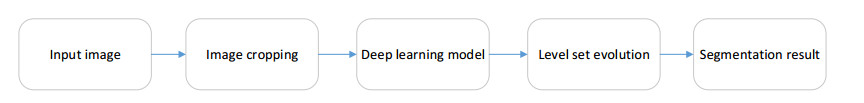
Accurate abdomen tissues segmentation is one of the crucial tasks in radiation therapy planning of related diseases. However, abdomen tissues segmentation (liver, kidney) is difficult because the low contrast between abdomen tissues and their surrounding organs. In this paper, an attention-based deep learning method for automated abdomen tissues segmentation is proposed. In our method, image cropping is first applied to the original images. U-net model with attention mechanism is then constructed to obtain the initial abdomen tissues. Finally, level set evolution which consists of three energy terms is used for optimize the initial abdomen segmentation. The proposed model is evaluated across 470 subsets. For liver segmentation, the mean dice are 96.2 and 95.1% for the FLARE21 datasets and the LiTS datasets, respectively. For kidney segmentation, the mean dice are 96.6 and 95.7% for the FLARE21 datasets and the LiTS datasets, respectively. Experimental evaluation exhibits that the proposed method can obtain better segmentation results than other methods.
Citation: Zhaoxuan Gong, Jing Song, Wei Guo, Ronghui Ju, Dazhe Zhao, Wenjun Tan, Wei Zhou, Guodong Zhang. Abdomen tissues segmentation from computed tomography images using deep learning and level set methods[J]. Mathematical Biosciences and Engineering, 2022, 19(12): 14074-14085. doi: 10.3934/mbe.2022655
Accurate abdomen tissues segmentation is one of the crucial tasks in radiation therapy planning of related diseases. However, abdomen tissues segmentation (liver, kidney) is difficult because the low contrast between abdomen tissues and their surrounding organs. In this paper, an attention-based deep learning method for automated abdomen tissues segmentation is proposed. In our method, image cropping is first applied to the original images. U-net model with attention mechanism is then constructed to obtain the initial abdomen tissues. Finally, level set evolution which consists of three energy terms is used for optimize the initial abdomen segmentation. The proposed model is evaluated across 470 subsets. For liver segmentation, the mean dice are 96.2 and 95.1% for the FLARE21 datasets and the LiTS datasets, respectively. For kidney segmentation, the mean dice are 96.6 and 95.7% for the FLARE21 datasets and the LiTS datasets, respectively. Experimental evaluation exhibits that the proposed method can obtain better segmentation results than other methods.

| [1] | O. Abd-Elaziz, M. Sayed, M. Abdullah, Liver tumors segmentation from abdominal CT images using region growing and morphological processing, in International Conference on Engineering and Technology (ICET), 2015. https://doi.org/10.1109/ICEngTechnol.2014.7016813 |
| [2] | S. Rafiei, N. Karimi, B. Mirmahboub, K. Najarian, S. Soroushmehr, Liver segmentation in abdominal CT images using probabilistic atlas and adaptive 3D region growing, in 2019 41st Annual International Conference of the IEEE Engineering in Medicine and Biology Society (EMBC), 2019. https://doi.org/10.1109/EMBC.2019.8857835 |
| [3] |
S. Tran, C. Cheng, D. Liu, A multiple layer U-Net, Un-Net, for liver and liver tumor segmentation in CT, IEEE Access, 9 (2020), 3752–3764. https://doi.org/10.1109/ACCESS.2020.3047861 doi: 10.1109/ACCESS.2020.3047861

|
| [4] |
P. Sofia, A. Juan, S. Manuel, A. Roberto, M. Alicia, D. Maceira, Automatic multi-atlas liver segmentation and couinaud classification from CT volumes, Annu. Int. Conf. IEEE Eng. Med. Biol. Soc., 2021 (2021), 2826–2829. https://doi.org/10.1109/EMBC46164.2021.9630668 doi: 10.1109/EMBC46164.2021.9630668
|
| [5] |
L. Song, H. Wang, Z. Wang, Bridging the gap between 2D and 3D contexts in CT volume for liver and tumor segmentation, IEEE J. Biomed. Health Inf., 9 (2021), 3450–3459. https://doi.org/10.1109/JBHI.2021.3075752 doi: 10.1109/JBHI.2021.3075752
|
| [6] | J. Zhang, B. Ji, Z. Jiang, J. Qin, CR-UNet: Context-rich UNet for liver segmentation from CT volumes, in 2021 International Conference on Electronic Information Engineering and Computer Science (EIECS), 2021. https://doi.org/10.1109/EIECS53707.2021.9588086 |
| [7] |
T. Lei, R. Wang, Y. Zhang, A. Nandi, DefED-Net: Deformable encoder-decoder network for liver and liver tumor segmentation, IEEE Trans. Radiat. Plasma Med. Sci., 6 (2022), 68–78. https://doi.org/10.1109/TRPMS.2021.3059780 doi: 10.1109/TRPMS.2021.3059780
|
| [8] |
X. Fang, S. Xu, B. Wood, P. Yan, Deep learning-based liver segmentation for fusion-guided intervention, Int. J. Comput. Assisted Radiol. Surg., 15 (2020), 963–972. https://doi.org/10.1007/s11548-020-02147-6 doi: 10.1007/s11548-020-02147-6
|
| [9] | T. Amina, L. Lakhdar, B. Hakim, M. Abdallah, Improved active contour model through automatic initialisation: Liver segmentation, in 2021 IEEE 1st International Maghreb Meeting of the Conference on Sciences and Techniques of Automatic Control and Computer Engineering MI-STA, 2021. https://doi.org/10.1109/MI-STA52233.2021.9464516 |
| [10] | M. N. U. Haq, A. Irtaza, N. Nida, M. A. Shah, L. Zubair, Liver tumor segmentation using resnet based mask-R-CNN, in 2021 International Bhurban Conference on Applied Sciences and Technologies (IBCAST), 2021. https://doi.org/10.1109/IBCAST51254.2021.9393194 |
| [11] |
X. Wang, Y. Zheng, G. Lan, W. Xuan, X. Sang, X. Kong, et al., Liver segmentation from CT images using a sparse priori statistical shape model (SP-SSM), PLoS One, 12 (2017), 1–23. https://doi.org/10.1371/journal.pone.0185249 doi: 10.1371/journal.pone.0185249
|
| [12] |
W. Qin, J. Wu, F. Han, Y. Yuan, W. Zhao, B. Ibragimov, et al., Superpixel-based and boundary-sensitive convolutional neural network for automated liver segmentation, Phys. Med. Biol., 9 (2018), 1–19. https://doi.org/10.1088/1361-6560/aabd19 doi: 10.1088/1361-6560/aabd19
|
| [13] | Y. Yao, Y. Sang, Z. Zhao, Y. Cao, Research on segmentation and recognition of liver CT image based on multi-scale feature fusion, in 2021 2nd International Symposium on Computer Engineering and Intelligent Communications (ISCEIC), 2021. https://doi.org/10.1109/ISCEIC53685.2021.00075 |
| [14] | S. Shao, X. Zhang, R. Cheng, C. Deng, Semantic segmentation method of 3D liver image based on contextual attention model, in 2021 IEEE International Conference on Systems, Man, and Cybernetics (SMC), 2021. https://doi.org/10.1109/SMC52423.2021.9659018 |
| [15] | C. Li, Y. Tan, W. Chen, X. Luo, Y. Gao, X. Jia, et al., Attention Unet++: A nested attention-aware U-Net for liver CT image segmentation, in 2020 IEEE International Conference on Image Processing (ICIP), 2020. https://doi.org/10.1109/ICIP40778.2020.9190761 |
| [16] | X. Yan, K. Yuan, W. Zhao, S. Wang, Z. Li, S. Cui, An efficient hybrid model for kidney tumor segmentation in CT images, in 2020 IEEE 17th International Symposium on Biomedical Imaging (ISBI), 2020. https://doi.org/10.1109/ISBI45749.2020.9098325 |
| [17] | N. Thein, A. Nugroho, T. Bharata, K Hamamoto, An image preprocessing method for kidney stone segmentation in CT scan images, in 2018 International Conference on Computer Engineering, Network and Intelligent Multimedia (CENIM), 2018. https://doi.org/10.1109/CENIM.2018.8710933 |
| [18] | G. Yang, G. Li, T. Pan, Y. Kong, X. Zhu, Automatic segmentation of kidney and renal tumor in CT images based on 3D fully convolutional neural network with pyramid pooling module, in 2018 24th International Conference on Pattern Recognition (ICPR), 2018. https://doi.org/10.1109/ICPR.2018.8545143 |
| [19] |
M. Arafat, G. Hamarne, R. Garbi, Cascaded regression neural nets for kidney localization and segmentation-free volume estimation, IEEE Trans. Med. Imaging, 40 (2021), 1555–1567. https://doi.org/10.1109/TMI.2021.3060465 doi: 10.1109/TMI.2021.3060465
|
| [20] | J. Chen, X. Zhang, J. Wang, Coarse-to-fine deformable model-based kidney 3D segmentation, in 2019 WRC Symposium on Advanced Robotics and Automation (WRC SARA), 2019. https://doi.org/10.1109/WRC-SARA.2019.8931969 |
| [21] | S. Yin, Z. Zhang, H. Li, Q. Peng, X. You, S. L. Furth, et al., Fully-automatic segmentation of kidneys in clinical ultrasound images using a boundary distance regression network, in 2019 IEEE 16th International Symposium on Biomedical Imaging (ISBI 2019), 2019. https://doi.org/10.1109/ISBI.2019.8759170 |
| [22] | R. Statkevych, S. Stirenko, Y. Gordienko, Human kidney tissue image segmentation by U-Net models, in IEEE EUROCON 2021-19th International Conference on Smart Technologies, 2021. https://doi.org/10.1109/EUROCON52738.2021.9535599 |
| [23] | M. Li, Y. Chen, X. Zheng, K. Liu, Kidney region of interest extraction based on iterative convolution threshold method, in 2021 6th International Conference on Communication, Image and Signal Processing (CCISP), 2021. https://doi.org/10.1109/CCISP52774.2021.9639090 |
| [24] |
T. Les, T. Markiewcz, M. Dziekiewicz, M. Lorent, Kidney segmentation from computed tomography images using U-Net and batch-based synthesis, Comput. Biol. Med., 123 (2020), 103906. https://doi.org/10.1016/j.compbiomed.2020.103906 doi: 10.1016/j.compbiomed.2020.103906
|
| [25] |
H. R. Torres, S. Queirós, P. Morais, B. Oliveira, J. Vilaca, Kidney segmentation in 3-D ultrasound images using a fast phase-based approach, IEEE Trans. Ultrason., Ferroelectr., Freq. Control, 68 (2021), 1521–1531. https://doi.org/10.1109/TUFFC.2020.3039334 doi: 10.1109/TUFFC.2020.3039334
|
| [26] |
N. Weerasinghe, N. Lovell, A. Welsh, G. Stevenson, Multi-parametric fusion of 3D power doppler ultrasound for fetal kidney segmentation using fully convolutional neural networks, IEEE J. Biomed. Health Inf., 25 (2021), 2050–2057. https://doi.org/10.1109/JBHI.2020.3027318 doi: 10.1109/JBHI.2020.3027318
|
| [27] | J. Guo, W. Zeng, S. Yu, J. Xiao, RAU-Net: U-Net model based on residual and attention for kidney and kidney tumor segmentation, in 2021 IEEE International Conference on Consumer Electronics and Computer Engineering (ICCECE), 2021. https://doi.org/10.1109/ICCECE51280.2021.9342530 |
| [28] | T. M. Geethanjali, Minavathi, M. S. Dinesh, Semantic segmentation of tumors in kidneys using attention U-Net models, international conference on electrical, in 2021 5th International Conference on Electrical, Electronics, Communication, Computer Technologies and Optimization Techniques (ICEECCOT), 2021. https://doi.org/10.1109/ICEECCOT52851.2021.9708025 |
| [29] |
C. Li, C. Xu, C. Gui, M. Fox, Distance regularized level set evolution and its application to image segmentation, IEEE Trans. Image Process., 19 (2010), 3243–3254. https://doi.org/10.1109/TIP.2010.2069690 doi: 10.1109/TIP.2010.2069690
|
| [30] |
T. Chan, L. Vese, Active contours without edges, IEEE Trans. Image Process., 10 (2001), 266–277. https://doi.org/10.1109/83.902291 doi: 10.1109/83.902291
|
| [31] |
C. Feng, D. Zhao, M. Huang, Image segmentation and bias correction using local inhomogeneous iNtensity clustering (LINC): A region-based level set method, Neurocomputing, 219 (2017), 107–129. https://doi.org/10.1016/j.neucom.2016.09.008 doi: 10.1016/j.neucom.2016.09.008
|
| [32] |
C. Li, C. Kao, J. Gore, Z. Ding, Minimization of region scalable fitting energy for image segmentation, IEEE Trans. Image Process., 17 (2008), 1940–1949. https://doi.org/10.1109/TIP.2008.2002304 doi: 10.1109/TIP.2008.2002304
|


Figures(6) / Tables(2)

Zhaoxuan Gong, Jing Song, Wei Guo, Ronghui Ju, Dazhe Zhao, Wenjun Tan, Wei Zhou, Guodong Zhang. Abdomen tissues segmentation from computed tomography images using deep learning and level set methods[J]. Mathematical Biosciences and Engineering, 2022, 19(12): 14074-14085. doi: 10.3934/mbe.2022655


 DownLoad: