Cutaneous squamous cell carcinoma (cSCC) is one of the most frequent types of cutaneous cancer. The composition and heterogeneity of the tumor microenvironment significantly impact patient prognosis and the ability to practice precision therapy. However, no research has been conducted to examine the design of the tumor microenvironment and its interactions with cSCC.
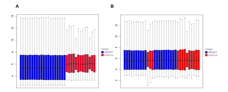
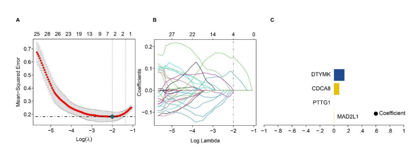
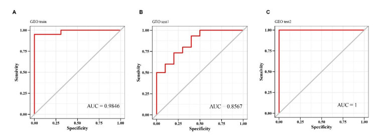
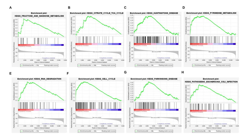
We retrieved the datasets GSE42677 and GSE45164 from the GEO public database, integrated them, and analyzed them using the SVA method. We then screened the core genes using the WGCNA network and LASSO regression and checked the model's stability using the ROC curve. Finally, we performed enrichment and correlation analyses on the core genes.
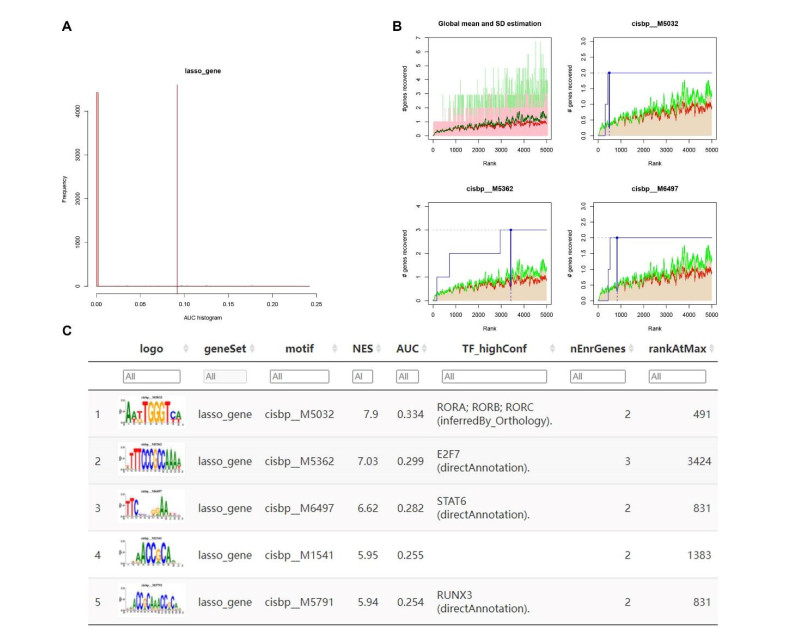
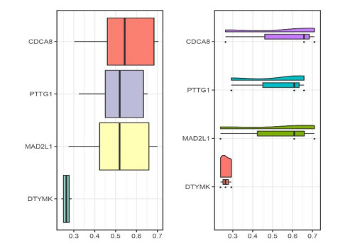
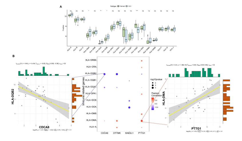
We identified four genes as core cSCC genes: DTYMK, CDCA8, PTTG1 and MAD2L1, and discovered that RORA, RORB and RORC were the primary regulators in the gene set. The GO semantic similarity analysis results indicated that CDCA8 and PTTG1 were the two most essential genes among the four core genes. The results of correlation analysis demonstrated that PTTG1 and HLA-DMA, CDCA8 and HLA-DQB2 were significantly correlated.
Examining the expression levels of four primary genes in cSCC aids in our understanding of the disease's pathophysiology. Additionally, the core genes were found to be highly related with immune regulatory genes, suggesting novel avenues for cSCC prevention and treatment.
Citation: Jiahua Xing, Muzi Chen, Yan Han. Multiple datasets to explore the tumor microenvironment of cutaneous squamous cell carcinoma[J]. Mathematical Biosciences and Engineering, 2022, 19(6): 5905-5924. doi: 10.3934/mbe.2022276
Cutaneous squamous cell carcinoma (cSCC) is one of the most frequent types of cutaneous cancer. The composition and heterogeneity of the tumor microenvironment significantly impact patient prognosis and the ability to practice precision therapy. However, no research has been conducted to examine the design of the tumor microenvironment and its interactions with cSCC.
We retrieved the datasets GSE42677 and GSE45164 from the GEO public database, integrated them, and analyzed them using the SVA method. We then screened the core genes using the WGCNA network and LASSO regression and checked the model's stability using the ROC curve. Finally, we performed enrichment and correlation analyses on the core genes.
We identified four genes as core cSCC genes: DTYMK, CDCA8, PTTG1 and MAD2L1, and discovered that RORA, RORB and RORC were the primary regulators in the gene set. The GO semantic similarity analysis results indicated that CDCA8 and PTTG1 were the two most essential genes among the four core genes. The results of correlation analysis demonstrated that PTTG1 and HLA-DMA, CDCA8 and HLA-DQB2 were significantly correlated.
Examining the expression levels of four primary genes in cSCC aids in our understanding of the disease's pathophysiology. Additionally, the core genes were found to be highly related with immune regulatory genes, suggesting novel avenues for cSCC prevention and treatment.

| [1] |
C. Fitzmaurice, D. Abate, N. Abbasi, H. Abbastabar, F. Abd-Allah, O. Abdel-Rahman, et al., Global, regional, and national cancer incidence, mortality, years of life lost, years lived with disability, and disability-adjusted life-years for 29 cancer groups, 1990 to 2017: a Systematic analysis for the global burden of disease study, JAMA Oncol., 5 (2019), 1749–1768. https://doi.org/10.1001/jamaoncol.2019.2996 doi: 10.1001/jamaoncol.2019.2996

|
| [2] |
H. Sung, J. Ferlay, R. L. Siegel, M. Laversanne, I. Soerjomataram, A. Jemal, et al., Global cancer statistics 2020: GLOBOCAN estimates of incidence and mortality worldwide for 36 cancers in 185 countries, CA Cancer J. Clin., 71 (2021), 209–249. https://doi.org/10.3322/caac.21660 doi: 10.3322/caac.21660
|
| [3] |
P. S. Karia, J. Han, C. D. Schmults, Cutaneous squamous cell carcinoma: estimated incidence of disease, nodal metastasis, and deaths from disease in the United States, 2012, J. Am. Acad. Dermatol., 68 (2013), 957–966. https://doi.org/10.1016/j.jaad.2012.11.037 doi: 10.1016/j.jaad.2012.11.037
|
| [4] |
J. M. Janus, R. F. L. O'Shaughnessy, C. Harwood, T. Maffucci, Phosphoinositide 3-Kinase-Dependent signalling pathways in cutaneous squamous cell carcinomas, Cancers, 9 (2017), 86. https://doi.org/10.3390/cancers9070086 doi: 10.3390/cancers9070086
|
| [5] |
M. Piipponen, R. Riihilä, L. Nissinen, V. Kähäri, The role of p53 in progression of cutaneous squamous cell carcinoma, Cancers, 13 (2021), 4507. https://doi.org/10.3390/cancers13184507 doi: 10.3390/cancers13184507
|
| [6] |
A. Boutros, F. Cecchi, E. Tanda, E. Croce, R. Gili1, L. Arecco, et al., Immunotherapy for the treatment of cutaneous squamous cell carcinoma, Front. Oncol., 11 (2021), 733917. https://doi.org/10.3389/fonc.2021.733917 doi: 10.3389/fonc.2021.733917
|
| [7] |
Y. Sawada, M. Nakamura, Daily lifestyle and cutaneous malignancies, Int. J. Mol. Sci., 22 (2021), 5227. https://doi.org/10.3390/ijms22105227 doi: 10.3390/ijms22105227
|
| [8] | K, Suozzi, J. Turban, M. Girardi, Cutaneous photoprotection: a review of the current status and evolving strategies, Yale J. Biol. Med., 93 (2020), 55–67. |
| [9] | C. Flower, D. Gaskin, S. Bhamjee, Z. Bynoe, High-risk variants of cutaneous squamous cell carcinoma in patients with discoid lupus erythematosus: a case series, Lupus, 22 (2013), 736–739. https://doi.org/10.1177%2F0961203313490243 |
| [10] |
K. K. Das, A. Chakaraborty, A. Rahman, S. Khandkar, Incidences of malignancy in chronic burn scar ulcers: experience from Bangladesh, Burns, 41 (2015), 1315–1321. https://doi.org/10.1016/j.burns.2015.02.008 doi: 10.1016/j.burns.2015.02.008
|
| [11] |
T. J. Knackstedt, L. K. Collins, Z. Li, S. Yan, F. Samie, Squamous cell carcinoma arising in hypertrophic lichen planus: a review and analysis of 38 cases, Dermatol. Surg., 41 (2015), 1411–1418. http://doi.org/10.1097/DSS.0000000000000565 doi: 10.1097/DSS.0000000000000565
|
| [12] |
J. Xing, Z. Jia, Y. Xu, M. Chen, Z. Yang, Y. Chen, et al., KLF9 (Kruppel Like Factor 9) induced PFKFB3 (6-Phosphofructo-2-Kinase/Fructose-2, 6-Biphosphatase 3) downregulation inhibits the proliferation, metastasis and aerobic glycolysis of cutaneous squamous cell carcinoma cells, Bioengineered, 12 (2021), 7563–7576. https://doi.org/10.1080/21655979.2021.1980644 doi: 10.1080/21655979.2021.1980644
|
| [13] |
J. G. Newman, M. A. Hall, S. J. Kurley, R. Cook, A. S. Farberg, J. L. Geiger, et al., Adjuvant therapy for high-risk cutaneous squamous cell carcinoma: 10-year review, Head Neck, 43 (2021), 2822–2843. https://doi.org/10.1002/hed.26767 doi: 10.1002/hed.26767
|
| [14] | J. Pang, H. Pan, C. Yang, P. Meng, W. Xie, J. Li, et al., Prognostic value of immune-related multi-incRNA signatures associated with tumor microenvironment in esophageal cancer, Front. Genet., 12 (2021), 722601. https://dx.doi.org/10.3389%2Ffgene.2021.722601 |
| [15] |
Y. Pan, H. Han, K. E. Labbe, H. Zhang, W. Wong, Recent advances in preclinical models for lung squamous cell carcinoma, Oncogene, 40 (2021), 2817–2829. https://doi.org/10.1038/s41388-021-01723-7 doi: 10.1038/s41388-021-01723-7
|
| [16] |
A. Elmusrati, J. Wang, C. Y. Wang, Tumor microenvironment and immune evasion in head and neck squamous cell carcinoma, Int. J. Oral. Sci., 13 (2021), 24. https://doi.org/10.1038/s41368-021-00131-7 doi: 10.1038/s41368-021-00131-7
|
| [17] |
T. Suwa, M. Kobayashi, J. M. Nam, H, Harada, Tumor microenvironment and radioresistance, Exp. Mol. Med., 53 (2021), 1029–1035. https://doi.org/10.1038/s12276-021-00640-9 doi: 10.1038/s12276-021-00640-9
|
| [18] | S. Paget, The distribution of secondary growths in cancer of the breast, Cancer Metastasis Rev., 8 (1889), 98–101. |
| [19] |
H. Wang, M. M. H. Yung, H. Y. S. Ngan, K. Chan, D. W. Chan, The impact of the tumor microenvironment on macrophage polarization in cancer metastatic progression, Int. J. Mol. Sci., 22 (2021), 6560. https://doi.org/10.3390/ijms22126560 doi: 10.3390/ijms22126560
|
| [20] |
J. Zhuyan, M. Chen, T. Zhu, X. Bao, T. Zhen, K. Xing, et al., Critical steps to tumor metastasis: alterations of tumor microenvironment and extracellular matrix in the formation of pre-metastatic and metastatic niche, Cell Biosci., 10 (2020), 89. https://doi.org/10.1186/s13578-020-00453-9 doi: 10.1186/s13578-020-00453-9
|
| [21] |
Y. Xie, F. Xie, L. Zhang, X. Zhou, J. Huang, F. Wang, et al., Targeted anti-tumor immunotherapy using tumor infiltrating cells, Adv. Sci., e2101672. https://doi.org/10.1002/advs.202101672 doi: 10.1002/advs.202101672
|
| [22] |
M. Akhtar, A. Haider, S. Rashid, A. Ai-Nabet, Paget's " Seed and Soil" theory of cancer metastasis: an idea whose time has come, Adv. Anat. Pathol., 26 (2019), 69–74. https://doi.org/10.1097/PAP.0000000000000219 doi: 10.1097/PAP.0000000000000219
|
| [23] |
G. Yan, L. Li, S. Zhu, Y. Wu, Y. Zhu, L. Zhu, et al., Single-cell transcriptomic analysis reveals the critical molecular pattern of UV-induced cutaneous squamous cell carcinoma, Cell Death Dis., 13 (2022), 23. https://doi.org/10.1038/s41419-021-04477-y doi: 10.1038/s41419-021-04477-y
|
| [24] |
A. Ji, A. Rubin, K. Thrane, S. Jiang, D. L. Reynolds, R. M. Meyers, et al., Multimodal analysis of composition and spatial architecture in human squamous cell carcinoma, Cell, 182 (2020), 497–514. https://doi.org/10.1016/j.cell.2020.05.039 doi: 10.1016/j.cell.2020.05.039
|
| [25] |
C. B. Steen, C. L. Liu, A. A. Alizadeh, A. M. Newman, Profiling cell type abundance and expression in bulk tissues with CIBERSORTx, Methods Mol. Biol., 2117 (2020), 135–157. https://doi.org/10.1007/978-1-0716-0301-7_7 doi: 10.1007/978-1-0716-0301-7_7
|
| [26] |
J. L. Sevilla, V. Segura, A. Podhorski, E. Guruceaga, J. M. Mato, L. A. Martinez-Cruz, et al., (2005) Correlation between gene expression and GO semantic similarity, IEEE/ACM Trans. Comput. Biol. Bioinform., 2 (2005), 330–338. https://doi.org/10.1109/TCBB.2005.50 doi: 10.1109/TCBB.2005.50
|
| [27] |
S. Jain, G. D. Bader, An improved method for scoring protein-protein interactions using semantic similarity within the gene ontology, BMC Bioinf., 11 (2010), 562. https://doi.org/10.1186/1471-2105-11-562 doi: 10.1186/1471-2105-11-562
|
| [28] | X. Guo, C. D. Shriver, H. Hu, M. N. Liebman, Analysis of metabolic and regulatory pathways through Gene Ontology-derived semantic similarity measures, in AMIA Annual Symposium Proceedings, American Medical Informatics Association, (2005), 972. |
| [29] |
P. M. Tedder, J. R. Bradford, C. J. Needham, G. A. McConkey, A. J. Bulpitt, D. R. Westhead, Gene function prediction using semantic similarity clustering and enrichment analysis in the malaria parasite Plasmodium falciparum, Bioinformatics, 26 (2010), 2431–2437. https://doi.org/10.1093/bioinformatics/btq450 doi: 10.1093/bioinformatics/btq450
|
| [30] |
G. Yu, F. Li, Y. Qin, X. Bo, Y. Wu, S. Wang, GOSemSim: an R package for measuring semantic similarity among GO terms and gene products, Bioinformatics, 26 (2010), 976–978. https://doi.org/10.1093/bioinformatics/btq064 doi: 10.1093/bioinformatics/btq064
|
| [31] |
J. Z. Wang, Z. Du, R. Payattakool, P. S. Yu, C. F. Chen, A new method to measure the semantic similarity of GO terms, Bioinformatics, 23 (2007), 1274–1281. https://doi.org/10.1093/bioinformatics/btm087 doi: 10.1093/bioinformatics/btm087
|
| [32] |
E. Rognoni, M. Widmaier, M. Jakobson, R. Ruppert, S. Ussar, D. Katsougkri, Kindlin-1 controls Wnt and TGF-β availability to regulate cutaneous stem cell proliferation, Nat. Med., 20 (2014), 350–359. https://doi.org/10.1038/nm.3490 doi: 10.1038/nm.3490
|
| [33] | M. Lai, R. Pampena, L. Cornacchia, G. Odorici, A. Piccerillo, G. Pellacani, et al., Cutaneous squamous cell carcinoma in patients with chronic lymphocytic leukemia: a systematic review of the literature, Int. J. Dermatol., 2021 (2021). https://doi.org/10.1111/ijd.15813 |
| [34] |
H. B. Jie, P. J. Schuler, S. C. Lee, R. M. Srivastava, A. Argiris, S. Ferrone, et al., CTLA-4⁺ regulatory T cells increased in cetuximab-treated head and neck cancer patients suppress NK cell cytotoxicity and correlate with poor prognosis, Cancer Res., 75 (2015), 2200–2210. https://doi.org/10.1158/0008-5472.CAN-14-2788 doi: 10.1158/0008-5472.CAN-14-2788
|
| [35] |
S. Z. Lin, K. J. Chen, Z. Y. Xu, H. Chen, L. Zhou, H. Y. Xie, et al., Prediction of recurrence and survival in hepatocellular carcinoma based on two Cox models mainly determined by FoxP3+ regulatory T cells, Cancer Prev. Res., 6 (2013), 594–602. https://doi.org/10.1158/1940-6207.CAPR-12-0379 doi: 10.1158/1940-6207.CAPR-12-0379
|
| [36] |
B. Azzimonti, E. Zavattaro, M. Provasi, M. Vidali, A. Conca, E. Catalano, et al., Intense Foxp3+ CD25+ regulatory T-cell infiltration is associated with high-grade cutaneous squamous cell carcinoma and counterbalanced by CD8+/Foxp3+ CD25+ ratio, Br. J. Dermatol., 172 (2014), 64–73. https://doi.org/10.1111/bjd.13172 doi: 10.1111/bjd.13172
|
| [37] | S. M. Gorsch, V. A. Memoli, T. A. Stukel, L. I. Gold, B. A. Arrick, Immunohistochemical staining for transforming growth factor beta 1 associates with disease progression in human breast cancer, Cancer Res., 52 (1992), 6949–6952. |
| [38] |
M. Ponzoni, F. Pastorino, D. Di Paolo, P. Perri, C. Brignole, Targeting macrophages as a potential therapeutic intervention: impact on inflammatory diseases and cancer, Int. J. Mol. Sci., 19 (2018), 1953. https://doi.org/10.3390/ijms19071953 doi: 10.3390/ijms19071953
|
| [39] |
L. Nissinen, M. Farshchian, P. Riihilä, V. Kähäre, New perspectives on role of tumor microenvironment in progression of cutaneous squamous cell carcinoma, Cell Tissue Res., 365 (2016), 691–702. https://doi.org/10.1007/s00441-016-2457-z doi: 10.1007/s00441-016-2457-z
|
| [40] |
J. S. Pettersen, J. Fuentes-Duculan, M. Suárez-Fariñas, K. C. Pierson, A. Pitts-Kiefer, L. Fan, et al., Tumor-associated macrophages in the cutaneous SCC microenvironment are heterogeneously activated, J. Invest. Dermatol., 131 (2011), 1322–1330. https://doi.org/10.1038/jid.2011.9 doi: 10.1038/jid.2011.9
|
| [41] |
M. Takahara, S. Chen, M. Kido, S. Takeuchi, H. Uchi, Y. Tu, et al., Stromal CD10 expression, as well as increased dermal macrophages and decreased Langerhans cells, are associated with malignant transformation of keratinocytes, J. Cutan. Pathol., 36 (2009), 668–674. https://doi.org/10.1111/j.1600-0560.2008.01139.x doi: 10.1111/j.1600-0560.2008.01139.x
|
| [42] |
D. Moussai, H. Mitsui, J. S. Pettersen, K. C. Pierson, K. R. Shah, M. Suárez- Fariñas, et al., The human cutaneous squamous cell carcinoma microenvironment is characterized by increased lymphatic density and enhanced expression of macrophage-derived VEGF-C, J. Invest. Dermatol., 131 (2011), 229–236. https://doi.org/10.1038/jid.2010.266 doi: 10.1038/jid.2010.266
|
| [43] | C. A. Janeway, J. Ron, M. E. Katz, The B cell is the initiating antigen-presenting cell in peripheral lymph nodes, J. Immunol., 138 (1987), 1051–1055. |
| [44] |
D. P. Harris, L. Haynes, P. C. Sayles, D. K. Duso, S. M. Eaton, N. M. Lepak, et al., Reciprocal regulation of polarized cytokine production by effector B and T cells, Nat. Immunol., 1 (2000), 475–482. https://doi.org/10.1038/82717 doi: 10.1038/82717
|
| [45] |
A. Sarvaria, J. A. Madrigal, A. Saudemont, B cell regulation in cancer and anti-tumor immunity, Cell Mol. Immunol., 14 (2017), 662–674. https://doi.org/10.1038/cmi.2017.35 doi: 10.1038/cmi.2017.35
|
| [46] |
P. Andreu, M. Johansson, N. Affara, F. Pucci, T. Tan, S. Junankar, et al., FcRgamma activation regulates inflammation-associated squamous carcinogenesis, Cancer Cell, 17 (2010), 121–134. https://doi.org/10.1016/j.ccr.2009.12.019 doi: 10.1016/j.ccr.2009.12.019
|
| [47] |
K. W. de Visser, L. V. Korets, L. M. Coussens, De novo carcinogenesis promoted by chronic inflammation is B lymphocyte dependent, Cancer Cell, 7 (2005), 411–423. https://doi.org/10.1016/j.ccr.2005.04.014 doi: 10.1016/j.ccr.2005.04.014
|
| [48] |
T. Schioppa, R. Moore, R. G. Thompson, F. R. Balkwill, B regulatory cells and the tumor-promoting actions of TNF-α during squamous carcinogenesis, Proc. Natl. Acad. Sci., 108 (2011), 10662–10667. https://doi.org/10.1073/pnas.1100994108 doi: 10.1073/pnas.1100994108
|
| [49] |
G. Crawford, M. D. Hayes, R. C. Seoane, S. Ward, T. Dalessandri, C. Lai, et al., Epithelial damage and tissue γδ T cells promote a unique tumor-protective IgE response, Nat. Immunol., 19 (2018), 859–870. https://doi.org/10.1038/s41590-018-0161-8 doi: 10.1038/s41590-018-0161-8
|
| [50] |
T. Zhou, R. Qin, S. Shi, H. Zhang, C. Niu, G. Ju, et al., DTYMK promote hepatocellular carcinoma proliferation by regulating cell cycle, Cell Cycle, 20 (2021), 1681–1691. https://doi.org/10.1080/15384101.2021.1958502 doi: 10.1080/15384101.2021.1958502
|
| [51] | Y. Guo, W. Luo, S. Huang, W. Zhao, H. Chen, Y. Ma, et al., DTYMK expression predicts prognosis and chemotherapeutic response and correlates with immune infiltration in hepatocellular carcinoma, J. Hepatocell Carcinoma, 8 (2021), 871–885. https://dx.doi.org/10.2147%2FJHC.S312604 |
| [52] |
T. Jeon, M. J. Ko, Y. R. Seo, S. J. Jung, D. Seo, S. Y. Park, et al., Silencing CDCA8 suppresses hepatocellular carcinoma growth and stemness via restoration of ATF3 tumor suppressor and inactivation of AKT/β-catenin signaling, Cancers, 13 (2021), 1055. https://doi.org/10.3390/cancers13051055 doi: 10.3390/cancers13051055
|
| [53] |
G. Vlotides, T. Eigler, S. Melmed, Pituitary tumor-transforming gene: physiology and implications for tumorigenesis, Endocr. Rev., 28 (2007), 165–186. https://doi.org/10.1210/er.2006-0042 doi: 10.1210/er.2006-0042
|
| [54] | H. Hong, Z. Jin, T. Qian, X. Xu, X. Zhu, Q. Fei, et al., Falcarindiol enhances cisplatin chemosensitivity of hepatocellular carcinoma via down-regulating the STAT3-modulated PTTG1 pathway, Front. Pharmacol., 12 (2021), 656697. https://dx.doi.org/10.3389%2Ffphar.2021.656697 |
| [55] |
S. W. Chen, H. F. Zhou, H. J. Zhang, R. He, Z. Huang, Y. Dang, et al., The clinical significance and potential molecular mechanism of PTTG1 in esophageal squamous cell carcinoma, Front. Genet., 11 (2021), 583085. https://doi.org/10.3389/fgene.2020.583085 doi: 10.3389/fgene.2020.583085
|
| [56] |
Z. Chen, K. Cao, Y. Hou, F. Lu, L. Li, L. Wang, et al., PTTG1 knockdown enhances radiation-induced antitumour immunity in lung adenocarcinoma, Life Sci., 277 (2021), 119594. https://doi.org/10.1016/j.lfs.2021.119594 doi: 10.1016/j.lfs.2021.119594
|
| [57] |
J. E. Noll, K. Vandyke, D. R. Hewett, K. M. Mrozik, R. J. Bala, S. A. Williams, et al., PTTG1 expression is associated with hyperproliferative disease and poor prognosis in multiple myeloma, J. Hematol. Oncol., 8 (2015), 106. https://doi.org/10.1186/s13045-015-0209-2 doi: 10.1186/s13045-015-0209-2
|
| [58] |
R. Wei, Z. Wang, Y. Zhang, B. Wang, N. Shen, E. Li, et al., Bioinformatic analysis revealing mitotic spindle assembly regulated NDC80 and MAD2L1 as prognostic biomarkers in non-small cell lung cancer development, BMC Med. Genomics, 13 (2020), 112. https://doi.org/10.1186/s12920-020-00762-5 doi: 10.1186/s12920-020-00762-5
|
| [59] |
M. Vleugel, T. A. Hoek, E. Tromer, T. Sliedrecht, V. Groenewold, M. Omerzu, et al., Dissecting the roles of human BUB1 in the spindle assembly checkpoint, J. Cell Sci., 128 (2015), 2975–2982. https://doi.org/10.1242/jcs.169821 doi: 10.1242/jcs.169821
|
| [60] |
Y. H. Ko, J. H. Roh, Y. I. Son, M. K. Chung, J. Y. Jang, H. Byun, et al., Expression of mitotic checkpoint proteins BUB1B and MAD2L1 in salivary duct carcinomas, J. Oral Pathol. Med., 39 (2010), 349–355. https://doi.org/10.1111/j.1600-0714.2009.00835.x doi: 10.1111/j.1600-0714.2009.00835.x
|
| [61] |
M. Abal, A. Obrador-Hevia, K. P. Janssen, L. Casadome, M. Menendez, S. Carpentier, et al., APC inactivation associates with abnormal mitosis completion and concomitant BUB1B/MAD2L1 up-regulation, Gastroenterology, 132 (2007), 2448–2458. https://doi.org/10.1053/j.gastro.2007.03.027 doi: 10.1053/j.gastro.2007.03.027
|
| [62] |
Y. Wang, Z. Zhou, L. Chen, Y. Li, Z. Zhou, X. Chu, Identification of key genes and biological pathways in lung adenocarcinoma via bioinformatics analysis, Mol. Cell Biochem., 476 (2021), 931–939. https://doi.org/10.1007/s11010-020-03959-5 doi: 10.1007/s11010-020-03959-5
|
| [63] |
R. Marima, R. Hull, C. Penny, Z. Dlamini, Mitotic syndicates Aurora Kinase B (AURKB) and mitotic arrest deficient 2 like 2 (MAD2L2) in cohorts of DNA damage response (DDR) and tumorigenesis, Mutat. Res. Rev. Mutat. Res., 787 (2021), 108376. https://doi.org/10.1016/j.mrrev.2021.108376 doi: 10.1016/j.mrrev.2021.108376
|
Figures(11)

Jiahua Xing, Muzi Chen, Yan Han. Multiple datasets to explore the tumor microenvironment of cutaneous squamous cell carcinoma[J]. Mathematical Biosciences and Engineering, 2022, 19(6): 5905-5924. doi: 10.3934/mbe.2022276


 DownLoad: