Photovoltaic models parameter estimation via an enhanced Rao-1 algorithm

Junhua Ku; Shuijia Li; Wenyin Gong; Junhua Ku; Shuijia Li; Wenyin Gong

doi:10.3934/mbe.2022052

Mathematical Biosciences and Engineering

2022, Volume 19, Issue 2: 1128-1153. doi: 10.3934/mbe.2022052

Previous Article Next Article

Research article Special Issues

Photovoltaic models parameter estimation via an enhanced Rao-1 algorithm

1.
School of Science, Qiongtai Normal University, Haikou, 571127, China
2.
School of Computer Science, China University of Geosciences, Wuhan 430074, China

Received: 18 October 2021 Accepted: 24 November 2021 Published: 30 November 2021

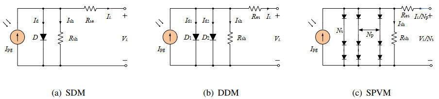
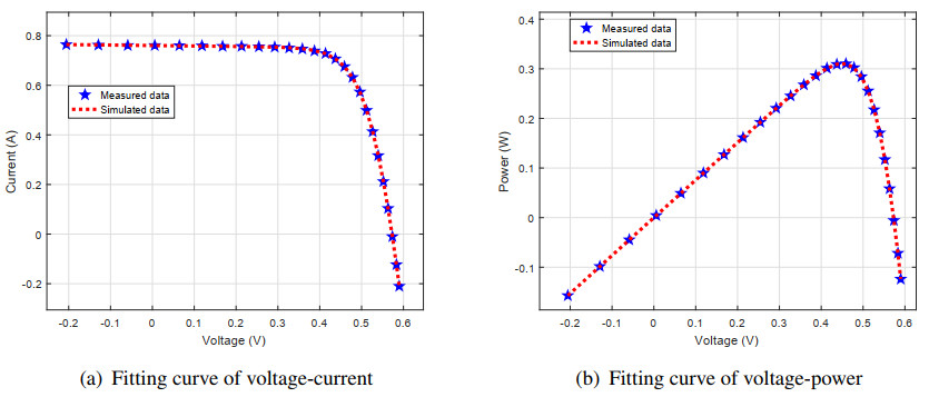
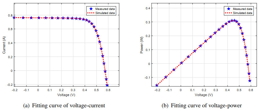
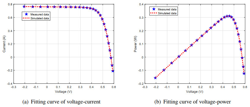
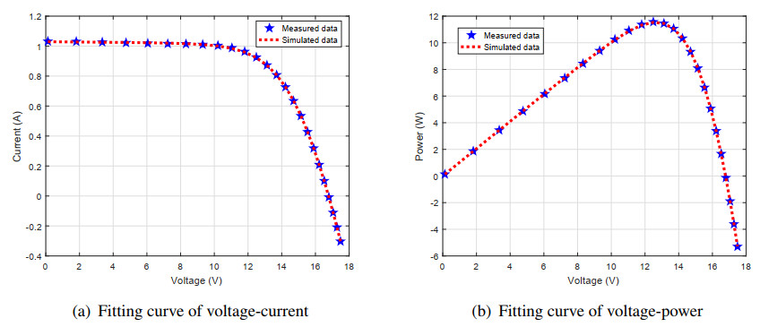
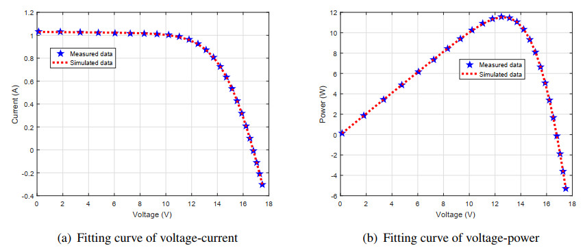
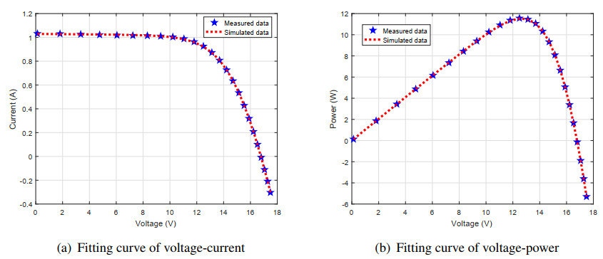
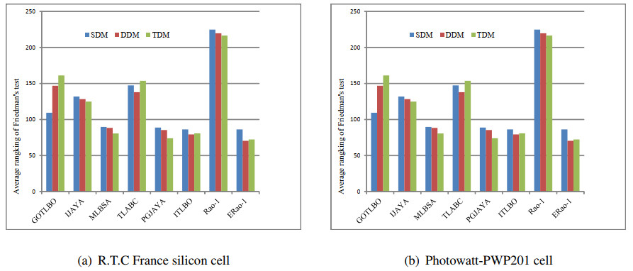
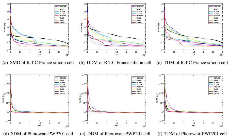
The accuracy of unknown parameters determines the accuracy of photovoltaic (PV) models that occupy an important position in the PV power generation system. Due to the complexity of the equation equivalent of PV models, estimating the parameters of the PV model is still an arduous task. In order to accurately and reliably estimate the unknown parameters in PV models, in this paper, an enhanced Rao-1 algorithm is proposed. The main point of enhancement lies in i) a repaired evolution operator is presented; ii) to prevent the Rao-1 algorithm from falling into a local optimum, a new evolution operator is developed; iii) in order to enable population size to change adaptively with the evolutionary process, the population size linear reduction strategy is employed. To verify the validity of ERao-1 algorithm, we embark a study on parameter estimation of three different PV models. Experimental results show that the proposed ERao-1 algorithm performs better than existing parameter estimation algorithms in terms of the accuracy and reliability, especially for the double diode model with RMSE 9.8248E-04, three diode model with RMSE 9.8257E-04 for the R.T.C France silicon cell, and 2.4251E-03 for the three diode model of Photowatt- PWP201 cell. In addition, the fitting curve of the simulated data and the measured data also shows the accuracy of the estimated parameters.

Keywords:

Citation: Junhua Ku, Shuijia Li, Wenyin Gong. Photovoltaic models parameter estimation via an enhanced Rao-1 algorithm[J]. Mathematical Biosciences and Engineering, 2022, 19(2): 1128-1153. doi: 10.3934/mbe.2022052

Related Papers:

[1]	Yuriĭ G. Nikonorov, Irina A. Zubareva . On the behavior of geodesics of left-invariant sub-Riemannian metrics on the group $ \operatorname{Aff}_{0}(\mathbb{R}) \times \operatorname{Aff}_{0}(\mathbb{R}) $. Electronic Research Archive, 2025, 33(1): 181-209. doi: 10.3934/era.2025010
[2]	Lakehal Belarbi . Ricci solitons of the $ \mathbb{H}^{2} \times \mathbb{R} $ Lie group. Electronic Research Archive, 2020, 28(1): 157-163. doi: 10.3934/era.2020010
[3]	Margarida Camarinha . A natural 4th-order generalization of the geodesic problem. Electronic Research Archive, 2024, 32(5): 3396-3412. doi: 10.3934/era.2024157
[4]	Wen Teng, Xiansheng Dai . Nonabelian embedding tensors on 3-Lie algebras and 3-Leibniz-Lie algebras. Electronic Research Archive, 2025, 33(3): 1367-1383. doi: 10.3934/era.2025063
[5]	Shanshan Liu, Abdenacer Makhlouf, Lina Song . The full cohomology, abelian extensions and formal deformations of Hom-pre-Lie algebras. Electronic Research Archive, 2022, 30(8): 2748-2773. doi: 10.3934/era.2022141
[6]	Hongliang Chang, Yin Chen, Runxuan Zhang . A generalization on derivations of Lie algebras. Electronic Research Archive, 2021, 29(3): 2457-2473. doi: 10.3934/era.2020124
[7]	Yizheng Li, Dingguo Wang . Lie algebras with differential operators of any weights. Electronic Research Archive, 2023, 31(3): 1195-1211. doi: 10.3934/era.2023061
[8]	Kailash C. Misra, Sutida Patlertsin, Suchada Pongprasert, Thitarie Rungratgasame . On derivations of Leibniz algebras. Electronic Research Archive, 2024, 32(7): 4715-4722. doi: 10.3934/era.2024214
[9]	Pengliang Xu, Xiaomin Tang . Graded post-Lie algebra structures and homogeneous Rota-Baxter operators on the Schrödinger-Virasoro algebra. Electronic Research Archive, 2021, 29(4): 2771-2789. doi: 10.3934/era.2021013
[10]	Shaban Khidr, Salomon Sambou . $ L^p $-theory for the $ {\partial }\overline{\partial} $-equation and isomorphisms results. Electronic Research Archive, 2025, 33(1): 68-86. doi: 10.3934/era.2025004

Abstract

1. Introduction

Einstein metrics are pivotal in numerous domains of mathematical physics and differential geometry. They are also of interest in pure mathematics, particularly in the fields of geometric analysis and algebraic geometry. An Einstein metric can be regarded as a fixed solution (up to diffeomorphism and scaling) of the Hamilton Ricci flow equation. On a Riemannian manifold $(M, g)$ , a Ricci soliton is said to exist when there is a smooth vector field $X$ and a constant $\lambda$ in the reals that satisfy the condition stated below:

$\begin{equation*} R_{ij}+\frac{1}{2}(\mathcal{L}_{X}g)_{ij} = \lambda g_{ij}, \end{equation*}$

where $R_{ij}$ is the Ricci curvature tensor, and $\mathcal{L}_{X}g$ stands for the Lie derivative of $g$ with respect to the vector field $X$ . This concept was introduced by Hamilton in ^[1], and later utilized by Perelman in his proof of the long-standing Poincare conjecture ^[2]. Lauret further generalized the notion of Einstein metrics to algebraic Ricci solitons in the Riemannian context, introducing them as a natural extension in ^[3]. Subsequently, Onda and Batat applied this framework to pseudo-Riemannian Lie groups, achieving a complete classification of algebraic Ricci solitons in three-dimensional Lorentzian Lie groups in ^[4]. Additionally, they proved that within the framework of pseudo-Riemannian manifolds, there is algebraic Ricci solitons that are not of the conventional Ricci soliton type.

In ^[5], Etayo and Santamaria explored the concept of distinguished connections on $(J^{2} = \pm1)$ -metric manifolds. This sparked interest among mathematicians in studying Ricci solitons linked to various affine connections, which can be found in ^[6,7,8]. The Bott connection was introduced in earlier works (see^[9,10,11]). In ^[12], the authors developed a theory on geodesic variations under metric changes in a geodesic foliation, with the Bott connection serving as the primary natural connection respecting the foliation's structure. In ^[13], Wu and Wang studied affine Ricci solitons and quasi-statistical structures on three-dimensional Lorentzian Lie groups associated with the Bott connection. Furthermore, in ^[14,15], the authors examined the algebraic schouten solitons and affine Ricci solitons concerning various affine connections.

Inspired by Lauret's work, Wears introduced algebraic T-solitons, linking them to T-solitons in ^[16]. Later, in ^[7], Azami introduced Schouten solitons, as a new type of generalized Ricci soliton. In this paper, I focus on algebraic Schouten solitons concerning the Bott connection with three distributions, aiming to classify and describe them on three-dimensional Lorentzian Lie groups.

In Section 2, I introduce the fundamental notions associated with three-dimensional Lie groups and algebraic Schouten soliton. In Sections 3–5, I discuss and present algebraic Schouten solitons concerning the Bott connection on three-dimensional Lorentzian Lie groups, each focusing on a different type of distribution.

2. Preliminaries

In ^[17], Milnor conducted a survey of both classical and recent findings on left-invariant Riemannian metrics on Lie groups, particularly on three-dimensional unimodular Lie groups. Furthermore, in ^[18], Rahmani classified three-dimensional unimodular Lie groups in the Lorentzian context. The non-unimodular cases were handled in ^[19,20]. Throughout this paper, I use $\{G_{i}\}_{i = 1}^{7}$ for connected, simply connected three-dimensional Lie groups equipped with a left-invariant Lorentzian metric $g$ . Their corresponding Lie algebras are denoted by $\{\mathfrak{g_{i}}\}_{i = 1}^{7}$ , and each possess a pseudo-orthonormal basis $\{e_{1}, e_{2}, e_{3}\}$ (with $e_{3}$ timelike, see ^[4]). Let $\nabla^{LC}$ and $R^{LC}$ denote the Levi-Civita connection and curvature tensor of $G_{i}$ , respectively, then

$\begin{equation*} R^{LC}(X,Y)Z = \nabla^{LC}_{X}\nabla^{LC}_{Y}Z-\nabla^{LC}_{Y}\nabla^{LC}_{X}Z-\nabla^{LC}_{[X,Y]}Z. \end{equation*}$

The Ricci tensor of $(G_{i}, g)$ is defined as follows:

$\begin{equation*} \rho^{LC}(X,Y) = -g(R^{LC}(X,e_{1})Y,e_{1})-g(R^{LC}(X,e_{2})Y,e_{2})+g(R^{LC}(X,e_{3})Y,e_{3}). \end{equation*}$

Moreover, I have the expression for the Ricci operator $Ric^{LC}$ :

$\begin{equation*} \rho^{LC}(X,Y) = g(Ric^{LC}(X),Y). \end{equation*}$

Next, recall the Bott connection, denoted by $\nabla^{B}$ . Consider a smooth manifold $(M, g)$ that is equipped with the Levi-Civita connection $\nabla$ , and let $TM$ represent its tangent bundle, spanned by $\{e_{1}, e_{2}, e_{3}\}$ . I introduce a distribution $D$ spanned by $\{e_{1}, e_{2}\}$ and its orthogonal complement $D^{\perp}$ , which is spanned by $\{e_{3}\}$ . The Bott connection $\nabla^{B}$ associated with distribution $D$ is then defined as follows:

$\begin{equation} \nabla_{X}^{B}Y = \left\{ \begin{aligned} &\pi_{D}(\nabla^{LC}_{X}Y),\quad X,Y\in\Gamma^{\infty}(D),\\ &\pi_{D}([X,Y]),\quad X\in\Gamma^{\infty}(D^{\perp}),\; Y\in\Gamma^{\infty}(D),\\ &\pi_{D^{\perp}}([X,Y]),\quad X\in\Gamma^{\infty}(D),\; Y\in\Gamma^{\infty}(D^{\perp}),\\ &\pi_{D^{\perp}}(\nabla^{LC}_{X}Y),\quad X,Y\in\Gamma^{\infty}(D^{\perp}), \end{aligned} \right. \end{equation}$

(2.1)

where $\pi_{D}$ (respectively, $\pi_{D^{\perp}}$ ) denotes the projection onto $D$ (respectively, $D^{\perp}$ ). For a more detailed discussion, refer to ^[9,10,11,21]. I denote the curvature tensor of the Bott connection $\nabla^{B}$ by $R^{B}$ , which is defined as follows:

$\begin{equation} R^{B}(X,Y)Z = \nabla^{B}_{X}\nabla^{B}_{Y}Z-\nabla^{B}_{Y}\nabla^{B}_{X}Z-\nabla^{B}_{[X,Y]}Z. \end{equation}$

(2.2)

The Ricci tensor $\rho^{B}$ associated to the connection $\nabla^{B}$ is defined as:

$\begin{equation*} \rho^{B}(X,Y) = \frac{B(X,Y)+B(Y,X)}{2}, \end{equation*}$

where

$\begin{equation*} B(X,Y) = -g(R^{B}(X,e_{1})Y,e_{1})-g(R^{B}(X,e_{2})Y,e_{2})+g(R^{B}(X,e_{3})Y,e_{3}). \end{equation*}$

Using the Ricci tensor $\rho^{B}$ , the Ricci operator $Ric^{B}$ is given by:

$\begin{equation} \rho^{B}(X,Y) = g(Ric^{B}(X),Y). \end{equation}$

(2.3)

Then, I have the definition of the Schouten tensor as follows:

$\begin{equation*} S^{B}(e_{i},e_{j}) = \rho^{B}(e_{i},e_{j})-\frac{s^{B}}{4}g(e_{i},e_{j}), \end{equation*}$

where $s^{B}$ represents the scalar curvature. Moreover, I generalized the Schouten tensor to:

$\begin{equation*} S^{B}(e_{i},e_{j}) = \rho^{B}(e_{i},e_{j})-s^{B}\lambda_{0}g(e_{i},e_{j}), \end{equation*}$

where $\lambda_{0}$ is a real number. By ^[22], I obtain the expression of $s^{B}$ as

$\begin{equation*} s^{B} = \rho^{B}(e_{1},e_{1})+\rho^{B}(e_{2},e_{2})-\rho^{B}(e_{3},e_{3}). \end{equation*}$

Definition 1. A manifold $(G_{i}, g)$ is called an algebraic Schouten soliton with associated to the connection $\nabla^{B}$ if it satisfies:

$\begin{equation*} Ric^{B} = (s^{B}\lambda_{0}+c)Id+D^{B}, \end{equation*}$

where $c$ is a constant, and $D^{B}$ is a derivation of $\mathfrak{g}_{i}$ , i.e.,

$\begin{equation} D^{B}[X_{1},X_{2}] = [D^{B}X_{1},X_{2}]+[X_{1},D^{B}X_{2}],\quad for\; X_{1},X_{2}\in \mathfrak{g}_{i}. \end{equation}$

(2.4)

3. Algebraic Schouten soliton concerning connection $\nabla^{B}$

In this section, I derive the algebraic criterion for the three-dimensional Lorentzian Lie group to exhibit an algebraic Schouten soliton related to the connection $\nabla^{B}$ . Moreover, I indicate that $G_{4}$ and $G_{7}$ do not have such solitons.

3.1. Algebraic Schouten soliton of $G_{1}$

According to ^[4], I have the expression for $\mathfrak{g}_{1}$ :

$\begin{equation*} [e_{1},e_{2}] = \alpha e_{1}-\beta e_{3},\quad [e_{1},e_{3}] = -\alpha e_{1}-\beta e_{2},\quad [e_{2},e_{3}] = \beta e_{1}+\alpha e_{2}+\alpha e_{3}, \end{equation*}$

where $\alpha\neq0$ . From this, I derive the following theorem.

Theorem 2. If $(G_{1}, g)$ constitutes an algebraic Schouten soliton concerning connection $\nabla^{B}$ ; then, it fulfills the conditions: $\beta = 0$ and $c = -\frac{1}{2}\alpha^{2}+2(\alpha^{2}+\beta^{2})\lambda_{0}$ .

Proof. From ^[23], the expression for $Ric^{B}$ is as follows:

$\begin{equation*} Ric^{B}\left( \begin{matrix} e_{1}\\ e_{2}\\ e_{3} \end{matrix}\right) = \left( \begin{matrix} -(\alpha^{2}+\beta^{2}) & \alpha\beta & \frac{1}{2}\alpha\beta\\ \alpha\beta & -(\alpha^{2}+\beta^{2}) & -\frac{1}{2}\alpha^{2}\\ -\frac{1}{2}\alpha\beta & \frac{1}{2}\alpha^{2} & 0 \end{matrix} \right) \left( \begin{matrix} e_{1}\\ e_{2}\\ e_{3} \end{matrix}\right). \end{equation*}$

The scalar curvature is $s^{B} = -2(\alpha^{2}+\beta^{2})$ . Now, I can express $D^{B}$ as follows:

$\begin{equation*} \left\{ \begin{aligned} &D^{B}e_{1} = -(\alpha^{2}+\beta^{2}+s\lambda_{0}+c)e_{1}+\alpha\beta e_{2}+\frac{\alpha\beta}{2}e_{3},\\ &D^{B}e_{2} = \alpha\beta e_{1}-(\alpha^{2}+\beta^{2}+s\lambda_{0}+c)e_{2}-\frac{\alpha^{2}}{2}e_{3},\\ &D^{B}e_{3} = -\frac{\alpha\beta}{2}e_{1}+\frac{\alpha^{2}}{2}e_{2}+(2(\alpha^{2}+\beta^{2})\lambda_{0}-c)e_{3}. \end{aligned} \right. \end{equation*}$

Therefore, based on Eq (2.4), there is an algebraic Schouten soliton associated with $\nabla^{B}$ on $(G_{1}, g)$ , if and only if the following condition satisfies:

$\begin{equation*} \left\{ \begin{aligned} &\frac{5}{2}\alpha^{2}\beta+2\beta^{3}-2\lambda_{0}\beta(\alpha^{2}+\beta^{2})+c\beta = 0,\\ &\frac{\alpha^{3}}{2}+2\alpha\beta^{2}-2\lambda_{0}\alpha(\alpha^{2}+\beta^{2})+c\alpha = 0,\\ &\alpha^{2}\beta = 0,\\ &2\alpha^{2}\beta+\beta^{3}-4\lambda_{0}\beta(\alpha^{2}+\beta^{2})+2c\beta = 0,\\ &\frac{\alpha^{3}}{2}+\frac{3}{2}\alpha\beta^{2}-2\lambda_{0}\alpha(\alpha^{2}+\beta^{2})+c\alpha = 0. \end{aligned} \right. \end{equation*}$

Since $\alpha\neq0$ , I have $\beta = 0$ and $c = -\frac{1}{2}\alpha^{2}+2(\alpha^{2}+\beta^{2})\lambda_{0}$ . □

3.2. Algebraic Schouten soliton of $G_{2}$

According to ^[4], I have the expression for $\mathfrak{g}_{2}$ :

$\begin{equation*} [e_{1},e_{2}] = \gamma e_{2}-\beta e_{3},\quad [e_{1},e_{3}] = -\beta e_{2}-\gamma e_{3},\quad [e_{2},e_{3}] = \alpha e_{1}, \end{equation*}$

where $\gamma\neq0$ . From this, I derive the following theorem.

Theorem 3. If $(G_{2}, g)$ constitutes an algebraic Schouten soliton concerning the connection $\nabla^{B}$ , then it fulfills the conditions: $\alpha = 0$ and $c = -\beta^{2}-\gamma^{2}+(\beta^{2}+2\gamma^{2})\lambda_{0}$ .

Proof. From ^[23], the expression for $Ric^{B}$ is as follows:

$\begin{equation*} Ric^{B}\left( \begin{matrix} e_{1}\\ e_{2}\\ e_{3} \end{matrix}\right) = \left( \begin{matrix} -(\beta^{2}+\gamma^{2}) & 0 & 0\\ 0 & -(\gamma^{2}+\alpha\beta) & \frac{\alpha\gamma}{2}\\ 0 & -\frac{\alpha\gamma}{2} & 0 \end{matrix} \right) \left( \begin{matrix} e_{1}\\ e_{2}\\ e_{3} \end{matrix}\right). \end{equation*}$

The scalar curvature is $s^{B} = -(\beta^{2}+2\gamma^{2}+\alpha\beta)$ . Now, I can express $D^{B}$ as follows:

$\begin{equation*} \left\{ \begin{aligned} &D^{B}e_{1} = -(\beta^{2}+\gamma^{2}-(\beta^{2}+2\gamma^{2}+\alpha\beta)\lambda_{0}+c)e_{1},\\ &D^{B}e_{2} = -(\gamma^{2}+\alpha\beta-(\beta^{2}+2\gamma^{2}+\alpha\beta)\lambda_{0}+c)e_{2}+\frac{\alpha\gamma}{2}e_{3},\\ &D^{B}e_{3} = -\frac{\alpha\gamma}{2}e_{2}+((\beta^{2}+2\gamma^{2}+\alpha\beta)\lambda_{0}-c)e_{3}. \end{aligned} \right. \end{equation*}$

Therefore, based on Eq (2.4), there is an algebraic Schouten soliton associated with $\nabla^{B}$ on $(G_{2}, g)$ , if and only if the following condition satisfies:

$\begin{equation*} \left\{ \begin{aligned} &\alpha\gamma^{2}-\beta^{3}+\alpha\beta^{2}+(\beta^{2}+2\gamma^{2}+\alpha\beta)\beta\lambda_{0}-c\beta = 0,\\ &\gamma(\beta^{2}+\gamma^{2}+\alpha\beta-(\beta^{2}+2\gamma^{2}+\alpha\beta)\lambda_{0}+c) = 0,\\ &\alpha\gamma^{2}-\beta^{3}-2\beta\gamma^{2}-\alpha\beta^{2}+(\beta^{2}+2\gamma^{2}+\alpha\beta)\beta\lambda_{0}-c\beta = 0,\\ &\alpha(-\beta^{2}+\alpha\beta-(\beta^{2}+2\gamma^{2}+\alpha\beta)\lambda_{0}+c) = 0. \end{aligned} \right. \end{equation*}$

Suppose that $\alpha = 0$ , then $c = -\beta^{2}-\gamma^{2}+(\beta^{2}+2\gamma^{2})\lambda_{0}$ . If $\alpha\neq0$ , I have

$\begin{equation*} \left\{ \begin{aligned} &\beta(\beta^{2}+\gamma^{2}-(\beta^{2}+2\gamma^{2}+\alpha\beta)\lambda_{0}+c) = 0,\\ &\beta^{2}+\gamma^{2}+\alpha\beta-(\beta^{2}+2\gamma^{2}+\alpha\beta)\lambda_{0}+c = 0,\\ &-\beta^{2}+\alpha\beta-(\beta^{2}+2\gamma^{2}+\alpha\beta)\lambda_{0}+c = 0. \end{aligned} \right. \end{equation*}$

Since $\gamma\neq0$ , solving the equations of the above system gives $2\beta^{2}+\gamma^{2} = 0$ , which is a contradiction. □

3.3. Algebraic Schouten soliton of $G_{3}$

According to ^[4], I have the expression for $\mathfrak{g}_{3}$ :

$\begin{equation*} [e_{1},e_{2}] = -\gamma e_{3},\quad [e_{1},e_{3}] = -\beta e_{2},\quad [e_{2},e_{3}] = \alpha e_{1}. \end{equation*}$

From this, I derive the following theorem.

Theorem 4. If $(G_{3}, g)$ is an algebraic Schouten soliton concerning connection $\nabla^{B}$ ; then, one of the following cases holds:

i. $\alpha = \beta = \gamma = 0$ , for all $c$ ;

ii. $\alpha\neq0$ , $\beta = \gamma = 0$ , $c = 0$ ;

iii. $\alpha = \gamma = 0$ , $\beta\neq0$ , $c = 0$ ;

iv. $\alpha\neq0$ , $\beta\neq0$ , $\gamma = 0$ , $c = 0$ ;

v. $\alpha = \beta = 0$ , $\gamma\neq0$ , $c = 0$ ;

vi. $\alpha\neq0$ , $\beta = 0$ , $\gamma\neq0$ , $c = -\alpha\gamma+\alpha\gamma\lambda_{0}$ ;

vii. $\alpha = 0$ , $\beta\neq0$ , $\gamma\neq0$ , $c = -\beta\gamma+\beta\gamma\lambda_{0}$ .

Proof. From ^[23], the expression for $Ric^{B}$ is as follows:

$\begin{equation*} Ric^{B}\left( \begin{matrix} e_{1}\\ e_{2}\\ e_{3} \end{matrix}\right) = \left( \begin{matrix} -\beta\gamma & 0 & 0\\ 0 & -\alpha\gamma & 0\\ 0 & 0 & 0 \end{matrix} \right) \left( \begin{matrix} e_{1}\\ e_{2}\\ e_{3} \end{matrix}\right). \end{equation*}$

The scalar curvature is $s^{B} = -\gamma(\alpha+\beta)$ . Now, I can express $D^{B}$ as follows:

$\begin{equation*} \left\{ \begin{aligned} &D^{B}e_{1} = -(\beta\gamma-\gamma(\alpha+\beta)\lambda_{0}+c)e_{1},\\ &D^{B}e_{2} = -(\alpha\gamma-\gamma(\alpha+\beta)\lambda_{0}+c)e_{2},\\ &D^{B}e_{3} = (\gamma(\alpha+\beta)\lambda_{0}-c)e_{3}. \end{aligned} \right. \end{equation*}$

Therefore, based on Eq (2.4), there is an algebraic Schouten soliton associated with $\nabla^{B}$ on $(G_{3}, g)$ , if and only if the following condition satisfies:

$\begin{equation} \left\{ \begin{aligned} &\beta\gamma^{2}+\alpha\gamma^{2}-\gamma^{2}(\alpha+\beta)\lambda_{0}+c\gamma = 0,\\ &\beta^{2}\gamma-\beta\gamma(\alpha+\beta)\lambda_{0}+c\beta = 0,\\ &\alpha^{2}\gamma-\alpha\beta\gamma-\alpha\gamma(\alpha+\beta)\lambda_{0}+c\alpha = 0. \end{aligned} \right. \end{equation}$

(3.1)

Assuming that $\gamma = 0$ . In this case, (3.1) becomes:

$\begin{equation} \left\{ \begin{aligned} &\beta c = 0,\\ &\alpha c = 0. \end{aligned} \right. \end{equation}$

(3.2)

If $\beta = 0$ , for Cases i and ii, system (3.1) holds. If $\beta\neq0$ , for Cases iii and iv, system (3.1) holds. Then, I assume that $\gamma\neq0$ . Thus, system (3.1) becomes:

$\begin{equation} \left\{ \begin{aligned} &\beta\gamma+\alpha\gamma-\gamma(\alpha+\beta)\lambda_{0}+c,\\ &\alpha \beta = 0. \end{aligned} \right. \end{equation}$

(3.3)

If $\beta = 0$ , I have Cases v and vi. If $\beta\neq0$ , for Case vii, system (3.1) holds □

3.4. Algebraic Schouten soliton of $G_{4}$

According to ^[4], $\mathfrak{g}_{4}$ takes the following form:

$\begin{equation*} [e_{1},e_{2}] = -e_{2}+(2\eta-\beta)e_{3},\quad [e_{1},e_{3}] = e_{3}-\beta e_{2},\quad [e_{2},e_{3}] = \alpha e_{1}, \end{equation*}$

where $\eta = 1\; or\; -1$ . From this, I derive the following theorem.

Theorem 5. $(G_{4}, g)$ is not an algebraic Schouten soliton concerning connection $\nabla^{B}$ .

Proof. According to ^[23], the expression for $Ric^{B}$ is derived as follows:

$\begin{equation*} Ric^{B}\left( \begin{matrix} e_{1}\\ e_{2}\\ e_{3} \end{matrix}\right) = \left( \begin{matrix} -(\beta-\eta)^{2} & 0 & 0\\ 0 & 2\alpha\eta-\alpha\beta-1 & -\frac{1}{2}\alpha\\ 0 & \frac{1}{2}\alpha & 0 \end{matrix} \right) \left( \begin{matrix} e_{1}\\ e_{2}\\ e_{3} \end{matrix}\right). \end{equation*}$

The scalar curvature is $s^{B} = -((\beta-\eta)^{2}+\alpha\beta-2\alpha\eta+1)$ . Now, I can express $D^{B}$ as follows:

$\begin{equation*} \left\{ \begin{aligned} &D^{B}e_{1} = -((\beta-\eta)^{2}-((\beta-\eta)^{2}+\alpha\beta-2\alpha\eta+1)\lambda_{0}+c)e_{1},\\ &D^{B}e_{2} = (2\alpha\eta-\alpha\beta-1+((\beta-\eta)^{2}+\alpha\beta-2\alpha\eta+1)\lambda_{0}-c)e_{2}-\frac{a}{2} e_{3},\\ &D^{B}e_{3} = \frac{\alpha}{2}e_{2}+(((\beta-\eta)^{2}+\alpha\beta-2\alpha\eta+1)\lambda_{0}-c)e_{3}. \end{aligned} \right. \end{equation*}$

Therefore, based on Eq (2.4), there is an algebraic Schouten soliton associated with $\nabla^{B}$ on $(G_{4}, g)$ , if and only if the following condition satisfies:

$\begin{equation} \left\{ \begin{aligned} &-(2\eta-\beta)((\beta-\eta)^{2}-2\alpha\eta+\alpha\beta+1-((\beta-\eta)^{2}+\alpha\beta-2\alpha\eta+1)\lambda_{0}+c) = \alpha,\\ &\beta((\beta-\eta)^{2}+2\alpha\eta-\alpha\beta-1-((\beta-\eta)^{2}+\alpha\beta-2\alpha\eta+1)\lambda_{0}+c) = \alpha,\\ &(\beta-\eta)^{2}-((\beta-\eta)^{2}+\alpha\beta-2\alpha\eta+1)\lambda_{0}+c = \alpha(\eta-\beta),\\ &\alpha((\beta-\eta)^{2}+2\alpha\eta-\alpha\beta-1+((\beta-\eta)^{2}+\alpha\beta-2\alpha\eta+1)\lambda_{0}-c) = 0. \end{aligned} \right. \end{equation}$

(3.4)

I now analyze the system under different assumptions.

Assuming that $\alpha = 0$ . Then, system (3.4) becomes:

$\begin{equation*} \left\{ \begin{aligned} &(2\eta-\beta)((\beta-\eta)^{2}+1-((\beta-\eta)^{2}+1)\lambda_{0}+c) = 0,\\ &\beta((\beta-\eta)^{2}-1-((\beta-\eta)^{2}+1)\lambda_{0}+c) = 0,\\ &(\beta-\eta)^{2}-((\beta-\eta)^{2}+1)\lambda_{0}+c = 0. \end{aligned} \right. \end{equation*}$

Upon direct calculation, it is evident that $(2\eta-\beta) = \beta = 0$ , which leads to a contradiction.

If $\alpha\neq0$ , we have

$\begin{equation} \left\{ \begin{aligned} &(2\eta-\beta)(\alpha\eta-1) = \alpha,\\ &\beta(3\alpha\eta-2\alpha\beta-1) = \alpha,\\ &(\beta-\eta)^{2}-\alpha(\eta-\beta)-((\beta-\eta)^{2}-2\alpha\eta+\alpha\beta+1)\lambda_{0}+c = 0,\\ &\alpha((\beta-\eta)^{2}+2\alpha\eta-\alpha\beta-1+((\beta-\eta)^{2}-2\alpha\eta+\alpha\beta+1)\lambda_{0}-c) = 0. \end{aligned} \right. \end{equation}$

(3.5)

From the last two equations in (3.5), we have $(\beta-\eta)^{2} = (1-\alpha\eta)$ . Substituting into the first two equations in (3.5) yields $\alpha = \eta$ , which is a contradiction. Therefore, system (3.4) has no solutions. Then, the theorem is true. □

3.5. Algebraic Schouten soliton of $G_{5}$

According to ^[4], we have the expression for $\mathfrak{g}_{5}$ :

$\begin{equation*} [e_{1},e_{2}] = 0,\quad [e_{1},e_{3}] = \alpha e_{1}+\beta e_{2},\quad [e_{2},e_{3}] = \gamma e_{1}+\delta e_{2}, \end{equation*}$

where $\alpha+\delta\neq0$ and $\alpha\gamma-\beta\delta = 0$ . From this, we derive the following theorem.

Theorem 6. If $(G_{5}, g)$ constitutes an algebraic Schouten soliton concerning connection $\nabla^{B}$ , then $c = 0$ .

Proof. According to ^[23], the expression for $Ric^{B}$ is derived as follows:

$\begin{equation*} Ric^{B}\left( \begin{matrix} e_{1}\\ e_{2}\\ e_{3} \end{matrix}\right) = \left( \begin{matrix} 0 & 0 & 0\\ 0 & 0 & 0\\ 0 & 0 & 0 \end{matrix} \right) \left( \begin{matrix} e_{1}\\ e_{2}\\ e_{3} \end{matrix}\right). \end{equation*}$

The scalar curvature is $s^{B} = 0$ . Now, I can express $D^{B}$ as follows:

$\begin{equation*} \left\{ \begin{aligned} &D^{B}e_{1} = -ce_{1},\\ &D^{B}e_{2} = -ce_{2},\\ &D^{B}e_{3} = -ce_{3}. \end{aligned} \right. \end{equation*}$

Hence, by (2.4), I conclude that there is an algebraic Schouten soliton associated with $\nabla^{B}$ on $(G_{5}, g)$ . Furthermore, for this algebraic Schouten soliton, I have $c = 0$ . □

3.6. Algebraic Schouten soliton of $G_{6}$

According to ^[4], I have the expression for $\mathfrak{g}_{6}$ :

$\begin{equation*} \begin{aligned} &[e_{1},e_{2}] = \alpha e_{2}+\beta e_{3},\\ &[e_{1},e_{3}] = \gamma e_{2}+\delta e_{3},\\ &[e_{2},e_{3}] = 0, \end{aligned} \end{equation*}$

where $\alpha+\delta\neq0$ and $\alpha\gamma-\beta\delta = 0$ . From this, I derive the following theorem.

Theorem 7. If $(G_{6}, g)$ constitutes an algebraic Schouten soliton concerning connection $\nabla^{B}$ , then one of the following cases holds:

i. $\alpha = \beta = \gamma = 0$ , $\delta\neq0$ , $c = 0$ ;

ii. $\alpha = \beta = 0$ , $\gamma\neq0$ , $\delta\neq0$ , $c = 0$ ;

iii. $\alpha\neq0$ , $\beta = \gamma = \delta = 0$ , $c = -\alpha^{2}+2\alpha^{2}\lambda_{0}$ ;

iv. $\alpha\neq0$ , $\beta = \gamma = 0$ , $\delta\neq0$ , $c = -\alpha^{2}+2\alpha^{2}\lambda_{0}$ .

Proof. From ^[23], I have the expression for $Ric^{B}$ as follows:

$\begin{equation*} Ric^{B}\left( \begin{matrix} e_{1}\\ e_{2}\\ e_{3} \end{matrix}\right) = \left( \begin{matrix} -(\alpha^{2}+\beta\gamma)^{2} & 0 & 0\\ 0 & -\alpha^{2} & 0\\ 0 & 0 & 0 \end{matrix} \right) \left( \begin{matrix} e_{1}\\ e_{2}\\ e_{3} \end{matrix}\right). \end{equation*}$

The scalar curvature is $s^{B} = -(2\alpha^{2}+\beta\gamma)$ . Now, I can express $D^{B}$ as follows:

$\begin{equation} \left\{ \begin{aligned} &D^{B}e_{1} = -(\alpha^{2}+\beta\gamma-(2\alpha^{2}+\beta\gamma)\lambda_{0}+c)e_{1},\\ &D^{B}e_{2} = -(\alpha^{2}-(2\alpha^{2}+\beta\gamma)\lambda_{0}+c)e_{2},\\ &D^{B}e_{3} = ((2\alpha^{2}+\beta\gamma)\lambda_{0}-c)e_{3}. \end{aligned} \right. \end{equation}$

(3.6)

Therefore, based on Eq (2.4), there is an algebraic Schouten soliton associated with $\nabla^{B}$ on $(G_{6}, g)$ , if and only if the following condition satisfies:

$\begin{equation*} \left\{ \begin{aligned} &\beta(2\alpha^{2}+\beta\gamma-(2\alpha^{2}+\beta\gamma)\lambda_{0}+c) = 0,\\ &\alpha(\alpha^{2}+\beta\gamma-(2\alpha^{2}+\beta\gamma)\lambda_{0}+c) = 0,\\ &\gamma(\beta\gamma-(2\alpha^{2}+\beta\gamma)\lambda_{0}+c) = 0,\\ &\delta(\alpha^{2}+\beta\gamma-(2\alpha^{2}+\beta\gamma)\lambda_{0}+c) = 0. \end{aligned} \right. \end{equation*}$

From the first equation above, we have either $\beta = 0$ or $\beta\neq0$ . I now analyze the system under different assumptions.

Assuming that $\beta = 0$ , I have:

$\begin{equation} \left\{ \begin{aligned} &\alpha(\alpha^{2}-2\alpha^{2}\lambda_{0}+c) = 0,\\ &\gamma(-2\alpha^{2}\lambda_{0}+c) = 0,\\ &\delta(\alpha^{2}-2\alpha^{2}\lambda_{0}+c) = 0. \end{aligned} \right. \end{equation}$

(3.7)

Given $\alpha\gamma-\beta\delta = 0$ and $\alpha+\delta\neq0$ , assume first that $\alpha = 0$ . In this case, system (3.7) can be simplified to:

$\begin{equation*} s^{B}\lambda_{0}+c = 0. \end{equation*}$

Then, I have Cases i and ii. If $\beta\neq0$ , system (3.7) becomes:

$\begin{equation} \alpha^{2}+s^{B}\lambda_{0}+c = 0. \end{equation}$

(3.8)

Then, I have Cases iii and iv.

If $\beta\neq0$ , system (3.7) becomes:

$\begin{equation} \left\{ \begin{aligned} &\beta(2\alpha^{2}+\beta\gamma-(2\alpha^{2}+\beta\gamma)\lambda_{0}+c) = 0,\\ &\alpha(\alpha^{2}+\beta\gamma-(2\alpha^{2}+\beta\gamma)\lambda_{0}+c) = 0, \end{aligned} \right. \end{equation}$

(3.9)

which is a contradiction. □

3.7. Algebraic Schouten soliton of $G_{7}$

According to ^[4], I have the expression for $\mathfrak{g}_{7}$ :

$\begin{equation*} \begin{aligned} &[e_{1},e_{2}] = -\alpha e_{1}-\beta e_{2}-\beta e_{3},\\ &[e_{1},e_{3}] = \alpha e_{1}+\beta e_{2}+\beta e_{3},\\ &[e_{2},e_{3}] = \gamma e_{1}+\delta e_{2}+\delta e_{3}, \end{aligned} \end{equation*}$

where $\alpha+\delta\neq0$ and $\alpha\delta = 0$ . From this, I derive the following theorem.

Theorem 8. $(G_{7}, g)$ is not an algebraic Schouten soliton concerning connection $\nabla^{B}$ .

Proof. From ^[23], I have the expression for $Ric^{B}$ as follows:

$\begin{equation*} Ric^{B}\left( \begin{matrix} e_{1}\\ e_{2}\\ e_{3} \end{matrix}\right) = \left( \begin{matrix} -\alpha^{2} & \frac{1}{2}\beta(\delta-\alpha) & -\delta(\alpha+\delta)\\ \frac{1}{2}\beta(\delta-\alpha) & -(\alpha^{2}+\beta^{2}+\beta\delta) & -\delta^{2}-\frac{1}{2}(\beta\gamma+\alpha\delta)\\ \delta(\alpha+\delta) & \delta^{2}+\frac{1}{2}(\beta\gamma+\alpha\delta) & 0 \end{matrix} \right) \left( \begin{matrix} e_{1}\\ e_{2}\\ e_{3} \end{matrix}\right). \end{equation*}$

The scalar curvature is $s^{B} = -(2\alpha^{2}+\beta^{2}+\beta\delta)$ . Now, I can express $D^{B}$ as follows:

$\begin{equation*} \left\{ \begin{array}{lll} D^{B}e_{1} = -(\alpha^{2}-(2\alpha^{2}+\beta^{2}+\beta\delta)\lambda_{0}+c)e_{1}+\frac{1}{2}\beta(\delta-\alpha)e_{2}-\delta(\alpha+\delta)e_{3},\\ D^{B}e_{2} = \frac{1}{2}\beta(\delta-\alpha)e_{1}-(\alpha^{2}+\beta^{2}+\beta\delta-(2\alpha^{2}+\beta^{2}+\beta\delta)\lambda_{0}+c)e_{2}-(\delta^{2}+\frac{1}{2}(\beta\gamma+\alpha\delta))e_{3},\\ D^{B}e_{3} = \delta(\alpha+\delta)e_{1}+(\delta^{2}+\frac{1}{2}(\beta\gamma+\alpha\delta))e_{2}+((2\alpha^{2}+\beta^{2}+\beta\delta)\lambda_{0}-c)e_{3}.\ \end{array} \right. \end{equation*}$

Therefore, based on Eq (2.4), there is an algebraic Schouten soliton associated with $\nabla^{B}$ on $(G_{7}, g)$ , if and only if the following condition satisfies:

$\begin{equation*} \left\{ \begin{array}{ll} \alpha(\alpha^{2}+\beta^{2}+\beta\alpha+s^{B}\lambda_{0}+c)+(\gamma+\beta)\delta(\alpha+\delta)+\frac{1}{2}\beta^{2}(\delta-\alpha) = \alpha(\delta^{2}+\frac{1}{2}(\beta\gamma+\alpha\delta)),\\ \beta(\alpha+s^{B}\lambda_{0}+c)+\delta^{2}(\alpha+\delta)+\frac{1}{2}\alpha\beta(\delta-\alpha) = 0,\\ \beta(2\alpha^{2}+\beta^{2}+\beta\alpha+s^{B}\lambda_{0}+c)+\delta(\delta-\alpha)(\alpha+\delta) = 2\beta(\delta^{2}+\frac{1}{2}(\beta\gamma+\alpha\delta)),\\ \alpha(s^{B}\lambda_{0}+c)+\alpha(\delta^{2}+\frac{1}{2}(\beta\gamma+\alpha\delta))+\frac{1}{2}\beta(\beta-\gamma)(\delta-\alpha)+\beta\delta(\alpha+\delta) = 0,\\ \beta(-\beta^{2}-\beta\alpha+s^{B}\lambda_{0}+c)-\frac{1}{2}\beta(\delta-\alpha)^{2}+2\beta(\delta^{2}+\frac{1}{2}(\beta\gamma+\alpha\delta)) = 0,\\ \beta(\alpha^{2}+s^{B}\lambda_{0}+c) = \alpha\delta(\alpha+\delta)+\frac{1}{2}\beta\delta(\delta-\alpha),\\ \gamma(\beta^{2}+\beta\alpha+s^{B}\lambda_{0}+c) = \delta(\alpha-\delta)(\alpha+\delta)-\frac{1}{2}\beta(\delta-\alpha)^{2},\\ \delta(s^{B}\lambda_{0}+c)+\delta(\delta^{2}+\frac{1}{2}(\beta\gamma+\alpha\delta)) = \beta\delta(\alpha+\delta)+\frac{1}{2}\beta(\delta-\alpha)(\beta-\gamma),\\ \delta(\alpha^{2}+\beta^{2}+\beta\alpha+s^{B}\lambda_{0}+c)-\delta(\delta^{2}+\frac{1}{2}(\beta\gamma+\alpha\delta)) = (\beta+\gamma)\delta(\alpha+\delta)+\frac{1}{2}\beta^{2}(\delta-\alpha). \end{array} \right. \end{equation*}$

Recall that $\alpha+\delta\neq0$ and $\alpha\gamma = 0$ . I now analyze the system under different assumptions:

Assume first that $\alpha\neq0$ , $\gamma = 0$ . Then, the above system becomes:

$\begin{equation} \left\{ \begin{array}{ll} \alpha(\alpha^{2}+\beta^{2}+\beta\alpha+s\lambda_{0}+c)+\beta\delta(\alpha+\delta)+\frac{1}{2}\beta^{2}(\delta-\alpha) = \alpha(\delta^{2}+\frac{1}{2}\alpha\delta),\\ \beta(\alpha+s\lambda_{0}+c)+\delta^{2}(\alpha+\delta)+\frac{1}{2}\alpha\beta(\delta-\alpha) = 0,\\ \beta(2\alpha^{2}+\beta^{2}+\beta\alpha+s\lambda_{0}+c)+\delta(\delta-\alpha)(\alpha+\delta) = 2\beta(\delta^{2}+\frac{1}{2}\alpha\delta),\\ \alpha(s\lambda_{0}+c)+\alpha(\delta^{2}+\frac{1}{2}\alpha\delta)+\frac{1}{2}\beta^{2}(\delta-\alpha)+\beta\delta(\alpha+\delta) = 0,\\ \beta(-\beta^{2}-\beta\alpha+s\lambda_{0}+c)-\frac{1}{2}\beta(\delta-\alpha)^{2}+2\beta(\delta^{2}+\frac{1}{2}\alpha\delta) = 0,\\ \beta(\alpha^{2}+s\lambda_{0}+c) = \alpha\delta(\alpha+\delta)+\frac{1}{2}\beta\delta(\delta-\alpha),\\ \delta(\alpha-\delta)(\alpha+\delta)-\frac{1}{2}\beta(\alpha-\delta)^{2} = 0,\\ \beta\delta(\alpha+\delta)+\frac{1}{2}\beta^{2}(\delta-\alpha) = \delta(s\lambda_{0}+c)+\delta(\delta^{2}+\frac{1}{2}\alpha\delta),\\ \beta\delta(\alpha+\delta)+\frac{1}{2}\beta^{2}(\delta-\alpha) = \delta(\alpha^{2}+\beta^{2}+\beta\alpha+s\lambda_{0}+c)-\delta(\delta^{2}+\frac{1}{2}\alpha\delta). \end{array} \right. \end{equation}$

(3.10)

Next, suppose that $\beta = 0$ , I have:

$\begin{equation} \left\{ \begin{aligned} &\alpha(\alpha^{2}+s\lambda_{0}+c)-\alpha(\delta^{2}+\frac{1}{2}\alpha\delta) = 0,\\ &\delta^{2}(\alpha+\delta) = 0. \end{aligned} \right. \end{equation}$

(3.11)

Which is a contradiction.

If $\beta\neq0$ , we further assume that $\delta = 0$ . Under this assumption, the last equation in (3.10) yields $\alpha^{2}\beta = 0$ , which leads to a contradiction. If we presume $\alpha = \delta$ , then the equations in (3.10) imply that $\alpha\delta(\alpha+\delta) = -\delta^{2}(\alpha+\delta)$ , which is a contradiction. Additionally, if I assume that $\delta\neq0$ and $\delta\neq-\alpha$ , then from equation system (3.10), I have the following equation:

$\begin{equation} \left\{ \begin{aligned} &\alpha^{2}+s\lambda_{0}+c = \frac{(\delta-\alpha)^{2}}{2},\\ &-\beta^{2}-\alpha\beta = \frac{(\delta-\alpha)^{2}}{2}-(\delta^{2}+\frac{\alpha\delta}{2}). \end{aligned} \right. \end{equation}$

(3.12)

Substituting (3.12) into the third equation in system (3.10) yields $\alpha^{2} = -\frac{1}{2}(\delta-\alpha)^{2}$ , which is a contradiction.

Second, let $\alpha = 0$ , $\gamma\neq0$ . Then, if $\beta = 0$ , the second equation in (3.10) reduces to $\delta^{3} = 0$ , which contradicts with $\alpha+\delta\neq0$ . On the other hand, if $\beta\neq0$ , I can derive from the second and sixth equations in system (3.10) that $\delta+\frac{1}{2}\beta = 0$ . Substituting into the fourth equation in (3.10) yields $\gamma = 0$ , which is a contradiction. □

4. Algebraic Schouten solitons concerning connection $\nabla^{B_{1}}$

In this section, I formulate the algebraic criterion necessary for a three-dimensional Lorentzian Lie group to have an algebraic Schouten soliton related to the Bott connection $\nabla^{B_{1}}$ . Recall the Bott connection, denoted by $\nabla^{B_{1}}$ , with the second distribution. Consider a smooth manifold $(M, g)$ that is equipped with the Levi-Civita connection $\nabla$ , and let $TM$ represent its tangent bundle, spanned by $\{e_{1}, e_{2}, e_{3}\}$ . I introduce a distribution $D_{1}$ spanned by $\{e_{1}, e_{3}\}$ and its orthogonal complement $D^{\perp}_{1}$ , which is spanned by $\{e_{2}\}$ . The Bott connection $\nabla^{B}_{1}$ associated with the distribution $D_{1}$ is then defined as follows:

$\begin{equation*} \nabla_{X}^{B_{1}}Y = \left\{ \begin{aligned} &\pi_{D_{1}}(\nabla^{LC}_{X}Y),\quad X,Y\in\Gamma^{\infty}(D_{1}),\\ &\pi_{D_{1}}([X,Y]),\quad X\in\Gamma^{\infty}(D_{1}^{\perp}),\; Y\in\Gamma^{\infty}(D_{1}),\\ &\pi_{D_{1}^{\perp}}([X,Y]),\quad X\in\Gamma^{\infty}(D_{1}),\; Y\in\Gamma^{\infty}(D_{1}^{\perp}),\\ &\pi_{D_{1}^{\perp}}(\nabla^{LC}_{X}Y),\quad X,Y\in\Gamma^{\infty}(D_{1}^{\perp}), \end{aligned} \right. \end{equation*}$

where $\pi_{D_{1}}$ (respectively, $\pi_{D_{1}^{\perp}}$ ) denotes the projection onto $D_{1}$ (respectively, $D_{1}^{\perp}$ ).

4.1. Algebraic Schouten soliton of $G_{1}$

Lemma 9. ^[13] The Ricci tensor $\rho^{B_{1}}$ concerning connection $\nabla^{B_{1}}$ of $(G_{1}, g)$ is given by:

$\begin{equation} \rho^{B_{1}}(e_{i},e_{j}) = \left( \begin{matrix} \alpha^{2}-\beta^{2} & \frac{1}{2}\alpha\beta & -\alpha\beta\\ \frac{1}{2}\alpha\beta & 0 & \frac{1}{2}\alpha^{2}\\ -\alpha\beta & \frac{1}{2}\alpha^{2} & \beta^{2}-\alpha^{2} \end{matrix} \right). \end{equation}$

(4.1)

From this, I derive the following theorem.

Theorem 10. If $(G_{1}, g)$ constitutes an algebraic Schouten soliton concerning connection $\nabla^{B_{1}}$ , then it fulfills the conditions: $\beta = 0$ and $c = \frac{1}{2}\alpha^{2}-2\alpha^{2}\lambda_{0}$ .

Proof. According to (4.1), the expression for $Ric^{B_{1}}$ is derived as follows:

$\begin{equation*} Ric^{B_{1}}\left( \begin{matrix} e_{1}\\ e_{2}\\ e_{3} \end{matrix}\right) = \left( \begin{matrix} \alpha^{2}-\beta^{2} & \frac{1}{2}\alpha\beta & \alpha\beta\\ \frac{1}{2}\alpha\beta & 0 & -\frac{1}{2}\alpha^{2}\\ -\alpha\beta & \frac{1}{2}\alpha^{2} & \alpha^{2}-\beta^{2} \end{matrix} \right) \left( \begin{matrix} e_{1}\\ e_{2}\\ e_{3} \end{matrix}\right). \end{equation*}$

The scalar curvature is $s^{B_{1}} = 2(\alpha^{2}-\beta^{2})$ . Now, I can express $D^{B_{1}}$ as follows:

$\begin{equation*} \left\{ \begin{aligned} &D^{B_{1}}e_{1} = (\alpha^{2}-\beta^{2}-2(\alpha^{2}-\beta^{2})\lambda_{0}-c)e_{1}+\frac{1}{2}\alpha\beta e_{2}+\alpha\beta e_{3},\\ &D^{B_{1}}e_{2} = \frac{1}{2}\alpha\beta e_{1}-(2(\alpha^{2}-\beta^{2})\lambda_{0}+c)e_{2}-\frac{\alpha^{2}}{2}e_{3},\\ &D^{B_{1}}e_{3} = -\alpha\beta e_{1}+\frac{1}{2}\alpha^{2} e_{2}+(\alpha^{2}-\beta^{2}-2(\alpha^{2}-\beta^{2})\lambda_{0}-c)e_{3}. \end{aligned} \right. \end{equation*}$

Therefore, based on Eq (2.4), there is an algebraic Schouten soliton associated with $\nabla^{B_{1}}$ on $(G_{1}, g)$ , if and only if the following condition satisfies:

$\begin{equation} \left\{ \begin{aligned} &\alpha(2(\alpha^{2}-\beta^{2})\lambda_{0}+c)+2\alpha\beta^{2}-\frac{1}{2}\alpha^{3} = 0,\\ &\alpha^{2}\beta = 0,\\ &\beta(2(\alpha^{2}-\beta^{2})\lambda_{0}+c)-2\alpha^{2}\beta = 0,\\ &\alpha(\alpha^{2}-\beta^{2}-2(\alpha^{2}-\beta^{2})\lambda_{0}-c)-\alpha\beta^{2}-\frac{1}{2}\alpha^{3} = 0,\\ &\beta(\alpha^{2}-2\beta^{2}-2(\alpha^{2}-\beta^{2})\lambda_{0}-c) = 0,\\ &\alpha(2(\alpha^{2}-\beta^{2})\lambda_{0}+c)-\frac{1}{2}\alpha^{3}+2\alpha\beta^{2} = 0. \end{aligned} \right. \end{equation}$

(4.2)

Since $\alpha\neq0$ , the second equation in (4.2) yields $\beta = 0$ . Then, I have $c = \frac{1}{2}\alpha^{2}-2\alpha^{2}\lambda_{0}$ . □

4.2. Algebraic Schouten soliton of $G_{2}$

Lemma 11. ^[13] The Ricci tensor $\rho^{B_{1}}$ concerning the connection $\nabla^{B_{1}}$ of $(G_{2}, g)$ is given by:

$\begin{equation} \rho^{B_{1}}(e_{i},e_{j}) = \left( \begin{matrix} -(\beta^{2}+\gamma^{2}) & 0 & 0\\ 0 & 0 & -\frac{1}{2}\alpha\gamma\\ 0 & -\frac{1}{2}\alpha\gamma & \alpha\beta+\gamma^{2} \end{matrix} \right). \end{equation}$

(4.3)

From this, I derive the following theorem.

Theorem 12. If $(G_{2}, g)$ constitutes an algebraic Schouten soliton concerning connection $\nabla^{B_{1}}$ ; then, it fulfills the conditions: $\alpha = \beta = 0$ and $c = -\gamma^{2}+\gamma^{2}\lambda_{0}$ .

Proof. According to (4.3), the expression for $Ric^{B_{1}}$ is derived as follows:

$\begin{equation*} Ric^{B_{1}}\left( \begin{matrix} e_{1}\\ e_{2}\\ e_{3} \end{matrix}\right) = \left( \begin{matrix} -(\beta^{2}+\gamma^{2}) & 0 & 0\\ 0 & 0 & \frac{1}{2}\alpha\gamma\\ 0 & -\frac{1}{2}\alpha\gamma & -\alpha\beta-\gamma^{2} \end{matrix} \right) \left( \begin{matrix} e_{1}\\ e_{2}\\ e_{3} \end{matrix}\right). \end{equation*}$

The scalar curvature is $s^{B_{1}} = -(\beta^{2}+\gamma^{2}+\alpha\beta)$ . Now, I can express $D^{B_{1}}$ as follows:

$\begin{equation*} \left\{ \begin{aligned} &D^{B_{1}}e_{1} = -(\beta^{2}+\gamma^{2}-(\beta^{2}+\gamma^{2}+\alpha\beta)\lambda_{0}+c)e_{1},\\ &D^{B_{1}}e_{2} = ((\beta^{2}+\gamma^{2}+\alpha\beta)\lambda_{0}-c)e_{2}+\frac{1}{2}\alpha\gamma e_{3},\\ &D^{B_{1}}e_{3} = -\frac{1}{2}\alpha\gamma e_{2}-(\alpha\beta+\gamma^{2}-(\beta^{2}+\gamma^{2}+\alpha\beta)\lambda_{0}+c)e_{3}. \end{aligned} \right. \end{equation*}$

Therefore, based on Eq (2.4), there is an algebraic Schouten soliton associated with $\nabla^{B_{1}}$ on $(G_{2}, g)$ , if and only if the following condition satisfies:

$\begin{equation} \left\{ \begin{aligned} &\alpha(\beta^{2}+\gamma^{2}-(\beta^{2}+\gamma^{2}+\alpha\beta)\lambda_{0}+c)+\frac{1}{2}\alpha\beta\gamma = 0,\\ &\beta((\beta^{2}+\gamma^{2}+\alpha\beta)\lambda_{0}-c)+\alpha\gamma^{2} = 0,\\ &\beta(\beta^{2}+2\gamma^{2}+\alpha\beta-(\beta^{2}+\gamma^{2}+\alpha\beta)\lambda_{0}+c)-\alpha\gamma^{2} = 0,\\ &\gamma(\beta^{2}+\gamma^{2}-(\beta^{2}+\gamma^{2}+\alpha\beta)\lambda_{0}+c)+\frac{1}{2}\alpha\beta\gamma = 0,\\ &\alpha(\alpha\beta-\beta^{2}-(\beta^{2}+\gamma^{2}+\alpha\beta)\lambda_{0}+c) = 0. \end{aligned} \right. \end{equation}$

(4.4)

By solving (4.4), I get $\alpha = \beta = 0$ , $c = -\gamma^{2}+\gamma^{2}\lambda_{0}$ . □

4.3. Algebraic Schouten soliton of $G_{3}$

Lemma 13. ^[13] The Ricci tensor $\rho^{B_{1}}$ concerning connection $\nabla^{B_{1}}$ of $(G_{3}, g)$ is given by:

$\begin{equation} \rho^{B_{1}}(e_{i},e_{j}) = \left( \begin{matrix} -\beta\gamma & 0 & 0\\ 0 & 0 & 0\\ 0 & 0 & \alpha\beta \end{matrix} \right). \end{equation}$

(4.5)

From this, I derive the following theorem.

Theorem 14. If $(G_{3}, g)$ constitutes an algebraic Schouten soliton concerning connection $\nabla^{B_{1}}$ ; then, one of the following cases holds:

i. $\alpha = \beta = \gamma = 0$ , for all $c$ ;

ii. $\alpha\neq0$ , $\beta = \gamma = 0$ , $c = 0$ ;

iii. $\alpha = 0$ , $\beta\neq0$ , $\gamma = 0$ , $c = 0$ ;

iv. $\alpha\neq0$ , $\beta\neq0$ , $\gamma = 0$ , $c = \alpha\beta\lambda_{0}$ ;

v. $\alpha = \beta = 0$ , $\gamma\neq0$ , $c = 0$ , ;

vi. $\alpha\neq0$ , $\beta = 0$ , $\gamma\neq0$ , $c = 0$ ;

vii. $\alpha = 0$ , $\beta\neq0$ , $\gamma\neq0$ , $c = -\beta\gamma+\beta\gamma\lambda_{0}$ .

Proof. According to (4.5), the expression for $Ric^{B_{1}}$ is derived as follows:

$\begin{equation*} Ric^{B_{1}}\left( \begin{matrix} e_{1}\\ e_{2}\\ e_{3} \end{matrix}\right) = \left( \begin{matrix} -\beta\gamma & 0 & 0\\ 0 & 0 & 0\\ 0 & 0 & -\alpha\beta \end{matrix} \right) \left( \begin{matrix} e_{1}\\ e_{2}\\ e_{3} \end{matrix}\right). \end{equation*}$

The scalar curvature is $s^{B_{1}} = -(\beta\gamma+\alpha\beta)$ . Now, I can express $D^{B_{1}}$ as follows:

$\begin{equation*} \left\{ \begin{aligned} &D^{B_{1}}e_{1} = -(\beta\gamma-(\beta\gamma+\alpha\beta)\lambda_{0}+c)e_{1},\\ &D^{B_{1}}e_{2} = ((\beta\gamma+\alpha\beta)\lambda_{0}-c)e_{2},\\ &D^{B_{1}}e_{3} = -(\alpha\beta-(\beta\gamma+\alpha\beta)\lambda_{0}+c)e_{3}. \end{aligned} \right. \end{equation*}$

Therefore, based on Eq (2.4), there is an algebraic Schouten soliton associated with $\nabla^{B_{1}}$ on $(G_{3}, g)$ , if and only if the following condition satisfies:

$\begin{equation} \left\{ \begin{aligned} &\gamma(\beta\gamma-\alpha\beta-(\beta\gamma+\alpha\beta)\lambda_{0}+c) = 0,\\ &\beta(\alpha\beta+\beta\gamma-(\beta\gamma+\alpha\beta)\lambda_{0}+c) = 0,\\ &\alpha(\alpha\beta-\beta\gamma-(\beta\gamma+\alpha\beta)\lambda_{0}+c) = 0. \end{aligned} \right. \end{equation}$

(4.6)

Assume first that $\gamma = 0$ ; then, (4.6) reduces to:

$\begin{equation*} \left\{ \begin{aligned} &\beta(\alpha\beta-\alpha\beta\lambda_{0}+c) = 0,\\ &\alpha(\alpha\beta-\alpha\beta\lambda_{0}+c) = 0. \end{aligned} \right. \end{equation*}$

Then, I have Cases i–iv.

Now, let $\gamma\neq0$ . From the last two equations in (4.6), I obtain $\alpha\beta\gamma = 0$ . If $\beta = 0$ , then it follows that $c = 0$ . Therefore, Cases v and vi are valid. If $\beta\neq0$ , we deduce $c = -\beta\gamma+\beta\gamma\lambda_{0}$ ; then, for Case vii, system (4.6) holds. □

4.4. Algebraic Schouten soliton of $G_{4}$

Lemma 15. ^[13] The Ricci tensor $\rho^{B_{1}}$ concerning connection $\nabla^{B_{1}}$ of $(G_{4}, g)$ is given by:

$\begin{equation} \rho^{B_{1}}(e_{i},e_{j}) = \left( \begin{matrix} -(\beta-\eta)^{2} & 0 & 0\\ 0 & 0 & \frac{1}{2}\alpha\\ 0 & \frac{1}{2}\alpha & \alpha\beta+1 \end{matrix} \right). \end{equation}$

(4.7)

From this, I derive the following theorem.

Theorem 16. If $(G_{4}, g)$ constitutes an algebraic Schouten soliton concerning connection $\nabla^{B_{1}}$ ; then, it fulfills the conditions: $\beta = \eta$ , $\alpha = -\beta$ and $c = 0$ .

Proof. According to (4.7), the expression for $Ric^{B_{1}}$ is derived as follows:

$\begin{equation*} Ric^{B_{1}}\left( \begin{matrix} e_{1}\\ e_{2}\\ e_{3} \end{matrix}\right) = \left( \begin{matrix} -(\beta-\eta)^{2} & 0 & 0\\ 0 & 0 & -\frac{1}{2}\alpha\\ 0 & \frac{1}{2}\alpha & -\alpha\beta-1 \end{matrix} \right) \left( \begin{matrix} e_{1}\\ e_{2}\\ e_{3} \end{matrix}\right). \end{equation*}$

The scalar curvature is $s^{B_{1}} = -((\beta-\eta)^{2}+\alpha\beta+1)$ . Now, I can express $D^{B_{1}}$ as follows:

$\begin{equation*} \left\{ \begin{aligned} &D^{B_{1}}e_{1} = -((\beta-\eta)^{2}-((\beta-\eta)^{2}+\alpha\beta+1)\lambda_{0}+c)e_{1},\\ &D^{B_{1}}e_{2} = (((\beta-\eta)^{2}+\alpha\beta+1)\lambda_{0}-c)e_{2}-\frac{1}{2}\alpha e_{3},\\ &D^{B_{1}}e_{3} = \frac{1}{2}\alpha-(\alpha\beta+1-((\beta-\eta)^{2}+\alpha\beta+1)\lambda_{0}+c)e_{3}. \end{aligned} \right. \end{equation*}$

Therefore, based on Eq (2.4), there is an algebraic Schouten soliton associated with $\nabla^{B_{1}}$ on $(G_{4}, g)$ , if the following condition satisfies:

$\begin{equation} \left\{ \begin{aligned} &(\beta-\eta)^{2}-((\beta-\eta)^{2}+\alpha\beta+1)\lambda_{0}+c-\alpha(\eta-\beta) = 0,\\ &(2\eta-\beta)((\beta-\eta)^{2}-\alpha\beta-1-((\beta-\eta)^{2}+\alpha\beta+1)\lambda_{0}+c)+\alpha = 0,\\ &\beta((\beta-\eta)^{2}+\alpha\beta+1-((\beta-\eta)^{2}+\alpha\beta+1)\lambda_{0}+c)-\alpha = 0,\\ &\alpha(\alpha\beta+1-(\beta-\eta)^{2}-((\beta-\eta)^{2}+\alpha\beta+1)\lambda_{0}+c) = 0. \end{aligned} \right. \end{equation}$

(4.8)

By solving the above system, I obtain the solutions $\beta = \eta$ , $\alpha = -\beta$ and $c = 0$ . In this case, the theorem is true. □

4.5. Algebraic Schouten soliton of $G_{5}$

Lemma 17. ^[13] The Ricci tensor $\rho^{B_{1}}$ concerning connection $\nabla^{B_{1}}$ of $(G_{5}, g)$ is given by:

$\begin{equation} \rho^{B_{1}}(e_{i},e_{j}) = \left( \begin{matrix} \alpha^{2} & 0 & 0\\ 0 & 0 & 0\\ 0 & 0 & -(\beta\gamma+\alpha^{2}) \end{matrix} \right). \end{equation}$

(4.9)

From this, I derive the following result.

Theorem 18. If $(G_{5}, g)$ constitutes an algebraic Schouten soliton concerning connection $\nabla^{B_{1}}$ ; then, one of the following cases holds:

i. $\alpha = \beta = \gamma = 0$ , $c = 0$ ;

ii. $\alpha = \beta = 0$ , $\gamma\neq0$ , $c = 0$ ;

iii. $\alpha = 0$ , $\beta\neq0$ , $\gamma\neq0$ , $c = -\beta\gamma+\beta\gamma\lambda_{0}$ ;

iv. $\alpha\neq0$ , $\beta = \delta = \gamma = 0$ , $c = -\alpha^{2}-2\alpha^{2}\lambda_{0}$ ;

v. $\alpha\neq0$ , $\beta = \gamma = 0$ , $\delta\neq0$ , $c = \alpha^{2}-2\alpha^{2}\lambda_{0}$ .

Proof. From (4.9), I have the expression for $Ric^{B_{1}}$ as follows:

$\begin{equation*} Ric^{B_{1}}\left( \begin{matrix} e_{1}\\ e_{2}\\ e_{3} \end{matrix}\right) = \left( \begin{matrix} \alpha^{2} & 0 & 0\\ 0 & 0 & 0\\ 0 & 0 & (\beta\gamma+\alpha^{2}) \end{matrix} \right) \left( \begin{matrix} e_{1}\\ e_{2}\\ e_{3} \end{matrix}\right). \end{equation*}$

The scalar curvature is $s^{B_{1}} = (2\alpha^{2}+\beta\gamma)$ . Now, I can express $D^{B_{1}}$ as follows:

$\begin{equation*} \left\{ \begin{aligned} &D^{B_{1}}e_{1} = (\alpha^{2}-(2\alpha^{2}+\beta\gamma)\lambda_{0}-c),\\ &D^{B_{1}}e_{2} = -((2\alpha^{2}+\beta\gamma)\lambda_{0}+c)e_{2}\\ &D^{B_{1}}e_{3} = (\beta\gamma+\alpha^{2}-(2\alpha^{2}+\beta\gamma)\lambda_{0}-c)e_{3}. \end{aligned} \right. \end{equation*}$

Therefore, based on Eq (2.4), there exists an algebraic Schouten soliton associated to $\nabla^{B_{1}}$ on $(G_{5}, g)$ , if and only if the following condition satisfies:

$\begin{equation} \left\{ \begin{aligned} &\alpha(\beta\gamma+\alpha^{2}-(\beta\gamma+2\alpha^{2})\lambda_{0}-c) = 0,\\ &\beta(\beta\gamma+2\alpha^{2}-(\beta\gamma+2\alpha^{2})\lambda_{0}-c) = 0,\\ &\gamma(\beta\gamma-(\beta\gamma+2\alpha^{2})\lambda_{0}-c) = 0,\\ &\delta(\beta\gamma+\alpha^{2}-(\beta\gamma+2\alpha^{2})\lambda_{0}-c) = 0. \end{aligned} \right. \end{equation}$

(4.10)

Assume first that $\alpha = 0$ , so I have:

$\begin{equation} \left\{ \begin{aligned} &\beta(\beta\gamma-\beta\gamma\lambda_{0}-c) = 0,\\ &\gamma(\beta\gamma-\beta\gamma\lambda_{0}-c) = 0,\\ &\delta(\beta\gamma-\beta\gamma\lambda_{0}-c) = 0. \end{aligned} \right. \end{equation}$

(4.11)

Then, for Cases i–iii, system (4.10) holds.

Now, I let $\alpha\neq0$ . The second equation in (4.10) leads to $\beta = 0$ , then system (4.10) reduces to:

$\begin{equation} \left\{ \begin{aligned} &\alpha(\alpha^{2}-2\alpha^{2}\lambda_{0}-c) = 0,\\ &\gamma(2\alpha^{2}\lambda_{0}+c) = 0,\\ &\delta(\alpha^{2}-2\alpha^{2}\lambda_{0}-c) = 0. \end{aligned} \right. \end{equation}$

(4.12)

This proves that Cases iv and v hold. □

4.6. Algebraic Schouten soliton of $G_{6}$

Lemma 19. ^[13] The Ricci tensor $\rho^{B_{1}}$ concerning connection $\nabla^{B_{1}}$ of $(G_{6}, g)$ is given by:

$\begin{equation} \rho^{B_{1}}(e_{i},e_{j}) = \left( \begin{matrix} -(\delta^{2}+\beta\gamma) & 0 & 0\\ 0 & 0 & 0\\ 0 & 0 & \delta^{2} \end{matrix} \right). \end{equation}$

(4.13)

From this, I derive the following result.

Theorem 20. If $(G_{6}, g)$ constitutes an algebraic Schouten soliton concerning connection $\nabla^{B_{1}}$ ; then, one of the following cases holds:

1) $\alpha = \beta = \gamma = 0$ , $\delta\neq0$ , $c = -\delta^{2}+2\delta^{2}\lambda_{0}$ ;

2) $\alpha\neq0$ , $\beta = \delta = \gamma = 0$ , $c = 0$ ;

3) $\alpha\neq0$ , $\beta\neq0$ , $\delta = \gamma = 0$ , $c = 0$ ;

4) $\alpha\neq0$ , $\beta = \gamma = 0$ , $\delta\neq0$ , $c = -\delta^{2}+2\delta^{2}\lambda_{0}$ .

Proof. From (4.13), I have the expression for $Ric^{B_{1}}$ as follows:

$\begin{equation*} Ric^{B_{1}}\left( \begin{matrix} e_{1}\\ e_{2}\\ e_{3} \end{matrix}\right) = \left( \begin{matrix} -(\delta^{2}+\beta\gamma) & 0 & 0\\ 0 & 0 & 0\\ 0 & 0 & -\delta^{2} \end{matrix} \right) \left( \begin{matrix} e_{1}\\ e_{2}\\ e_{3} \end{matrix}\right). \end{equation*}$

The scalar curvature is $s^{B_{1}} = -(2\delta^{2}+\beta\gamma)$ . Now, I can express $D^{B_{1}}$ as follows:

$\begin{equation*} \left\{ \begin{aligned} &D^{B_{1}}e_{1} = -(\delta^{2}+\beta\gamma-(2\delta^{2}+\beta\gamma)\lambda_{0}+c)e_{1},\\ &D^{B_{1}}e_{2} = ((2\delta^{2}+\beta\gamma)\lambda_{0}-c)e_{2},\\ &D^{B_{1}}e_{3} = -(\delta^{2}-(2\delta^{2}+\beta\gamma)\lambda_{0}+c). \end{aligned} \right. \end{equation*}$

Therefore, based on Eq (2.4), there is an algebraic Schouten soliton associated with $\nabla^{B_{1}}$ on $(G_{6}, g)$ , if and only if the following condition satisfies:

$\begin{equation} \left\{ \begin{aligned} &\alpha(\delta^{2}+\beta\gamma-(2\delta^{2}+\beta\gamma)\lambda_{0}+c) = 0,\\ &\beta(\beta\gamma-(2\delta^{2}+\beta\gamma)\lambda_{0}+c) = 0,\\ &\gamma(2\delta^{2}+\beta\gamma-(2\delta^{2}+\beta\gamma)\lambda_{0}+c) = 0,\\ &\delta(\delta^{2}+\beta\gamma-(2\delta^{2}+\beta\gamma)\lambda_{0}+c) = 0. \end{aligned} \right. \end{equation}$

(4.14)

Assume first $\alpha = 0$ . Then, $\alpha+\delta\neq0$ and $\alpha\gamma-\beta\delta = 0$ leads to $\beta = 0$ and $\delta\neq0$ . Therefore, system (4.14) reduces to:

$\begin{equation} \left\{ \begin{aligned} &\gamma(2\delta^{2}-2\delta^{2}\lambda_{0}+c) = 0,\\ &\delta(\delta^{2}-2\delta^{2}\lambda_{0}+c) = 0. \end{aligned} \right. \end{equation}$

(4.15)

Then, for Case 1), system (4.14) holds.

Now, let $\alpha\neq0$ . Suppose $\delta = 0$ , from the equations in (4.14) I can derive that $\gamma = 0$ . Then, I have $c = 0$ . Consequently, I have Cases 2) and 3). If $\delta\neq0$ , the equations in (4.14) imply that $\gamma = 0$ . Substituting into the second equation in (4.14) leads to $\beta = 0$ . Then, we have 4). □

4.7. Algebraic Schouten soliton of $G_{7}$

Lemma 21. ^[13] The Ricci tensor $\rho^{B_{1}}$ concerning connection $\nabla^{B_{1}}$ of $(G_{7}, g)$ is given by:

$\begin{equation} \rho^{B_{1}}(e_{i},e_{j}) = \left( \begin{matrix} \alpha^{2} & \beta(\alpha+\delta) & \frac{1}{2}\beta(\delta-\alpha)\\ \beta(\alpha+\delta) & 0 & \delta^{2}+\frac{1}{2}(\beta\gamma+\alpha\delta)\\ \frac{1}{2}\beta(\delta-\alpha) & \delta^{2}+\frac{1}{2}(\beta\gamma+\alpha\delta) & \beta^{2}-\alpha^{2}-\beta\gamma \end{matrix} \right). \end{equation}$

(4.16)

From this, we derive the following theorem.

Theorem 22. If $(G_{7}, g)$ constitutes an algebraic Schouten soliton concerning connection $\nabla^{B_{1}}$ ; then, it fulfills the conditions: $\alpha = 2\delta$ , $\beta = \gamma = 0$ , $c = \frac{\alpha^{2}}{2}-2\alpha^{2}\lambda_{0}$ .

Proof. From (4.16), I have the expression for $Ric^{B_{1}}$ as follows:

$\begin{equation*} Ric^{B_{1}}\left( \begin{matrix} e_{1}\\ e_{2}\\ e_{3} \end{matrix}\right) = \left( \begin{matrix} \alpha^{2} & \beta(\alpha+\delta) & -\frac{1}{2}\beta(\delta-\alpha)\\ \beta(\alpha+\delta) & 0 & -\delta^{2}-\frac{1}{2}(\beta\gamma+\alpha\delta)\\ \frac{1}{2}\beta(\delta-\alpha) & \delta^{2}+\frac{1}{2}(\beta\gamma+\alpha\delta) & -\beta^{2}+\alpha^{2}+\beta\gamma \end{matrix} \right) \left( \begin{matrix} e_{1}\\ e_{2}\\ e_{3} \end{matrix}\right). \end{equation*}$

The scalar curvature is $s^{B_{1}} = 2\alpha^{2}-\beta^{2}+\beta\gamma$ . Now, I can express $D^{B_{1}}$ as follows:

$\begin{equation*} \left\{ \begin{array}{lll} D^{B_{1}}e_{1} = (\alpha^{2}-(2\alpha^{2}-\beta^{2}+\beta\gamma)\lambda_{0}-c)e_{1}+\beta(\alpha+\delta)e_{2}-\frac{1}{2}\beta(\delta-\alpha)e_{3},\\ D^{B_{1}}e_{2} = \beta(\alpha+\delta)e_{1}-((2\alpha^{2}-\beta^{2}+\beta\gamma)\lambda_{0}+c)e_{2}-(\delta^{2}+\frac{1}{2}(\beta\gamma+\alpha\delta))e_{3},\\ D^{B_{1}}e_{3} = \frac{1}{2}\beta(\delta-\alpha)e_{1}+(\delta^{2}+\frac{1}{2}(\beta\gamma+\alpha\delta))e_{2}+(\alpha^{2}-\beta^{2}+\beta\gamma-(2\alpha^{2}-\beta^{2}+\beta\gamma)\lambda_{0}-c)e_{3}. \end{array} \right. \end{equation*}$

Therefore, based on Eq (2.4), there is an algebraic Schouten soliton associated with $\nabla^{B_{1}}$ on $(G_{7}, g)$ , if and only if the following condition satisfies:

$\begin{equation} \left\{ \begin{array}{ll} \alpha(s^{B_{1}}\lambda_{0}+c)-\frac{1}{2}\beta(\beta+\gamma)(\delta-\alpha)-\beta^{2}(\alpha+\delta)-\alpha(\delta^{2}+\frac{1}{2}(\beta\gamma+\alpha\delta)) = 0,\\ \beta(-\alpha^{2}+s^{B_{1}}\lambda_{0}+c)+\frac{1}{2}\beta\delta(\delta-\alpha)+\alpha\beta(\alpha+\delta) = 0,\\ \beta(-\beta^{2}+\beta\gamma+s^{B_{1}}\lambda_{0}+c)+\frac{1}{2}\beta(\delta-\alpha)^{2}-2\beta(\delta^{2}+\frac{1}{2}(\beta\gamma+\alpha\delta)) = 0,\\ \alpha(\alpha^{2}+\beta\gamma-\beta^{2}-s^{B_{1}}\lambda_{0}-c)+\beta(\gamma-\beta)(\alpha+\delta)-\frac{\beta^{2}(\delta-\alpha)}{2}-\alpha(\delta^{2}+\frac{\beta\gamma+\alpha\delta}{2}) = 0,\\ \beta(2\alpha^{2}+\beta\gamma-\beta^{2}-s^{B_{1}}\lambda_{0}-c)+\beta(\delta-\alpha)(\alpha+\delta)-2\beta(\delta^{2}+\frac{\beta\gamma+\alpha\delta}{2}) = 0,\\ \beta(\alpha^{2}-s^{B_{1}}\lambda_{0}-c)+\beta\delta(\alpha+\delta)+\frac{1}{2}\alpha\beta(\delta-\alpha) = 0,\\ \gamma(-\beta^{2}+\beta\gamma-s^{B_{1}}\lambda_{0}-c)+\beta(\alpha-\delta)(\alpha+\delta)-\frac{1}{2}\beta(\alpha-\delta)^{2} = 0,\\ \delta(\alpha^{2}-\beta^{2}+\beta\gamma-s^{B_{1}}\lambda_{0}-c)+\beta(\beta-\gamma)(\alpha+\delta)+\frac{\beta^{2}(\delta-\alpha)}{2}-\delta(\delta^{2}+\frac{\beta\gamma+\alpha\delta}{2}) = 0,\\ -\delta(s^{B_{1}}\lambda_{0}+c)+\beta^{2}(\alpha+\delta)+\frac{1}{2}\beta(\beta+\gamma)(\delta-\alpha)+\delta(\delta^{2}+\frac{1}{2}(\beta\gamma+\alpha\delta)) = 0. \end{array} \right. \end{equation}$

(4.17)

Since $\alpha\gamma = 0$ and $\alpha+\delta\neq0$ , I now analyze the system under different assumptions.

First, if $\alpha = 0$ and $\gamma\neq0$ , from the equations above, and after simple calculation, we have $\beta = 0$ . Furthermore, the seventh and eighth equations imply that $\delta^{3} = 0$ , which leads to a contradiction.

Second, if $\alpha\neq0$ and $\gamma = 0$ . the seventh equation gives rise to three possible subcases: $\beta = 0$ , $\alpha = \delta$ , or $\alpha+3\delta = 0$ . Initially, let's assume $\beta = 0$ . In this case, the equations in system (4.17), imply that $(\alpha-2\delta)(\alpha+\delta) = 0$ , leading to $\alpha = 2\delta$ , and the theorem is true. Next, I consider the subcase where $\alpha = \delta$ and $\beta\neq0$ . Then, the fifth and sixth equations result in $4\alpha^{2}+\beta^{2} = 0$ , which leads to a contradiction. Additionally, I consider that $\alpha+3\delta = 0$ and $\beta\neq0$ . The first and last equations provide $(2\alpha^{2}-\beta^{2}+\beta\gamma)\lambda_{0}+c = 0$ . Substituting this into the third equation derives $\beta = 0$ , which leads to a contradiction.

Finally, if $\alpha = \gamma = 0$ . The first equation in system (4.17) leads to $\beta = 0$ . Then, using the equations in (4.17), we have $\delta^{3} = 0$ , which leads to a contradiction. □

5. Algebraic Schouten solitons concerning connection $\nabla^{B_{2}}$

In this section, I formulate the algebraic criterion necessary for a three-dimensional Lorentzian Lie group to have an algebraic Schouten soliton related to the given Bott connection $\nabla^{B_{2}}$ . Let us recall the Bott connection with the third distribution, denoted by $\nabla^{B_{2}}$ . Consider a smooth manifold $(M, g)$ that is equipped with the Levi-Civita connection $\nabla$ , and let $TM$ represent its tangent bundle, spanned by $\{e_{1}, e_{2}, e_{3}\}$ . I introduce a distribution $D_{2}$ spanned by $\{e_{2}, e_{3}\}$ and its orthogonal complement $D^{\perp}_{2}$ , which is spanned by $\{e_{1}\}$ . The Bott connection $\nabla^{B}_{2}$ associated with the distribution $D_{2}$ is then defined as follows:

$\begin{equation} \nabla_{X}^{B_{2}}Y = \left\{ \begin{aligned} &\pi_{D_{2}}(\nabla^{LC}_{X}Y),\quad X,Y\in\Gamma^{\infty}(D_{2}),\\ &\pi_{D_{2}}([X,Y]),\quad X\in\Gamma^{\infty}(D_{2}^{\perp}),\; Y\in\Gamma^{\infty}(D_{2}),\\ &\pi_{D_{2}^{\perp}}([X,Y]),\quad X\in\Gamma^{\infty}(D_{2}),\; Y\in\Gamma^{\infty}(D_{2}^{\perp}),\\ &\pi_{D_{2}^{\perp}}(\nabla^{LC}_{X}Y),\quad X,Y\in\Gamma^{\infty}(D_{2}^{\perp}), \end{aligned} \right. \end{equation}$

(5.1)

where $\pi_{D_{2}}$ (respectively, $\pi_{D_{2}^{\perp}}$ ) denotes the projection onto $D_{2}$ (respectively, $D_{2}^{\perp}$ ).

5.1. Algebraic Schouten soliton of $G_{1}$

Lemma 23. ^[13] The Ricci tensor $\rho^{B_{2}}$ concerning connection $\nabla^{B_{2}}$ of $(G_{1}, g)$ is given by:

$\begin{equation} \rho^{B_{2}}(e_{i},e_{j}) = \left( \begin{matrix} 0 & \frac{1}{2}\alpha\beta & -\frac{1}{2}\alpha\beta\\ \frac{1}{2}\alpha\beta & -\beta^{2} & 0\\ -\frac{1}{2}\alpha\beta & 0 & \beta^{2} \end{matrix} \right). \end{equation}$

(5.2)

From this, I derive the following theorem.

Theorem 24. If $(G_{1}, g)$ constitutes an algebraic Schouten soliton concerning connection $\nabla^{B_{2}}$ ; then, it fulfills the conditions: $\alpha\neq0$ , $\beta = 0$ and $c = 0$ .

Proof. According to (5.2), the expression for $Ric^{B_{2}}$ is derived as follows:

$\begin{equation*} Ric^{B_{2}}\left( \begin{matrix} e_{1}\\ e_{2}\\ e_{3} \end{matrix}\right) = \left( \begin{matrix} 0 & \frac{1}{2}\alpha\beta & \frac{1}{2}\alpha\beta\\ \frac{1}{2}\alpha\beta & -\beta^{2} & 0\\ -\frac{1}{2}\alpha\beta & 0 & -\beta^{2} \end{matrix} \right) \left( \begin{matrix} e_{1}\\ e_{2}\\ e_{3} \end{matrix}\right). \end{equation*}$

The scalar curvature is $s^{B_{2}} = -2\beta^{2}$ . Now, I can express $D^{B_{2}}$ as follows:

$\begin{equation*} \left\{ \begin{aligned} &D^{B_{2}}e_{1} = (2\beta^{2}\lambda_{0}-c)e_{1}+\frac{1}{2}\alpha\beta e_{2}+\frac{1}{2}\alpha\beta e_{3},\\ &D^{B_{2}}e_{2} = \frac{1}{2}\alpha\beta e_{1}-(\beta^{2}-2\beta^{2}\lambda_{0}+c)e_{2},\\ &D^{B_{2}}e_{3} = -\frac{1}{2}\alpha\beta e_{1}-(\beta^{2}-2\beta^{2}\lambda_{0}+c)e_{3}. \end{aligned} \right. \end{equation*}$

Therefore, based on Eq (2.4), there is an algebraic Schouten soliton associated with $\nabla^{B_{2}}$ on $(G_{1}, g)$ , if and only if the following condition satisfies:

$\begin{equation} \left\{ \begin{aligned} &\alpha(\beta^{2}-2\beta^{2}\lambda_{0}+c)+\alpha\beta^{2} = 0,\\ &\alpha^{2}\beta = 0,\\ &\alpha(-2\beta^{2}\lambda_{0}+c)-\alpha\beta^{2} = 0,\\ &\beta(-2\beta^{2}\lambda_{0}+c)+\alpha^{2}\beta = 0. \end{aligned} \right. \end{equation}$

(5.3)

By solving (5.3), I have $\alpha\neq0$ , $\beta = 0$ and $c = 0$ . □

5.2. Algebraic Schouten soliton of $G_{2}$

Lemma 25. ^[13] The Ricci tensor $\rho^{B_{2}}$ concerning connection $\nabla^{B_{2}}$ of $(G_{2}, g)$ is given by:

$\begin{equation} \rho^{B_{2}}(e_{i},e_{j}) = \left( \begin{matrix} 0 & 0 & 0\\ 0 & -\alpha\beta & -\alpha\gamma\\ 0 & -\alpha\gamma & \alpha\beta \end{matrix} \right). \end{equation}$

(5.4)

From this, I derive the following theorem.

Theorem 26. If $(G_{2}, g)$ constitutes an algebraic Schouten soliton concerning connection $\nabla^{B_{2}}$ ; then, one of the following cases holds:

1) $\alpha = 0$ , $\beta = 0$ , $c = 0$ ;

2) $\alpha = 0$ , $\beta\neq0$ , $c = 0$ .

Proof. From (5.4), I have the expression for $Ric^{B_{2}}$ as follows:

$\begin{equation*} Ric^{B_{2}}\left( \begin{matrix} e_{1}\\ e_{2}\\ e_{3} \end{matrix}\right) = \left( \begin{matrix} 0 & 0 & 0\\ 0 & -\alpha\beta & \alpha\gamma\\ 0 & -\alpha\gamma & -\alpha\beta \end{matrix} \right) \left( \begin{matrix} e_{1}\\ e_{2}\\ e_{3} \end{matrix}\right). \end{equation*}$

The scalar curvature is $s^{B_{2}} = -2\alpha\beta$ . Now, I can express $D^{B_{2}}$ as follows:

$\begin{equation*} \left\{ \begin{aligned} &D^{B_{2}}e_{1} = (2\alpha\beta\lambda_{0}-c)e_{1},\\ &D^{B_{2}}e_{2} = -(\alpha\beta-2\alpha\beta\lambda_{0}+c)e_{2}+\alpha\gamma e_{3},\\ &D^{B_{2}}e_{3} = -\alpha\gamma e_{2}-(\alpha\beta-2\alpha\beta\lambda_{0}+c)e_{3}. \end{aligned} \right. \end{equation*}$

Therefore, based on Eq (2.4), there is an algebraic Schouten soliton associated with $\nabla^{B_{2}}$ on $(G_{2}, g)$ , if and only if the following condition satisfies:

$\begin{equation} \left\{ \begin{aligned} &\gamma(-2\alpha\beta\lambda_{0}+c)-2\alpha\beta\gamma = 0,\\ &\beta(-2\alpha\beta\lambda_{0}+c)-2\alpha\gamma^{2} = 0,\\ &\alpha(2\alpha\beta-2\alpha\beta\lambda_{0}+c) = 0. \end{aligned} \right. \end{equation}$

(5.5)

Since $\gamma\neq0$ , I assume first that $\alpha = 0$ . Under this assumption, the first two equations in (5.5) yield $c = 0$ . Therefore, Cases 1) and 2) hold. Now, let $\alpha\neq0$ , then I have $\beta = 0$ , and the second equation in (5.5) becomes $2\alpha\gamma^{2} = 0$ , which is a contradiction. □

5.3. Algebraic Schouten soliton of $G_{3}$

Lemma 27. ^[13] The Ricci tensor $\rho^{B_{2}}$ concerning connection $\nabla^{B_{2}}$ of $(G_{3}, g)$ is given by:

$\begin{equation} \rho^{B_{2}}(e_{i},e_{j}) = \left( \begin{matrix} 0 & 0 & 0\\ 0 & 0 & 0\\ 0 & 0 & \alpha\beta \end{matrix} \right). \end{equation}$

(5.6)

From this, I derive the following theorem.

Theorem 28. If $(G_{3}, g)$ constitutes an algebraic Schouten soliton concerning connection $\nabla^{B_{2}}$ ; then, one of the following cases holds:

1) $\alpha = \beta = \gamma = 0$ , for all $c$ ;

2) $\alpha = \gamma = 0$ , $\beta\neq0$ , $c = 0$ ;

3) $\alpha\neq0$ , $\beta = \gamma = 0$ , $c = 0$ ;

4) $\alpha\neq0$ , $\beta\neq0$ , $\gamma = 0$ , $c = -\alpha\beta+\alpha\beta\lambda_{0}$ ;

5) $\alpha = \beta = 0$ , $\gamma\neq0$ , $c = 0$ .

Proof. According to (5.6), the expression for $Ric^{B_{2}}$ is derived as follows:

$\begin{equation*} Ric^{B_{2}}\left( \begin{matrix} e_{1}\\ e_{2}\\ e_{3} \end{matrix}\right) = \left( \begin{matrix} 0 & 0 & 0\\ 0 & 0 & 0\\ 0 & 0 & -\alpha\beta \end{matrix} \right) \left( \begin{matrix} e_{1}\\ e_{2}\\ e_{3} \end{matrix}\right). \end{equation*}$

The scalar curvature is $s^{B_{2}} = -\alpha\beta$ . Now, I can express $D^{B_{2}}$ as follows:

$\begin{equation} \left\{ \begin{aligned} &D^{B_{2}}e_{1} = (\alpha\beta\lambda_{0}-c)e_{1},\\ &D^{B_{2}}e_{2} = (\alpha\beta\lambda_{0}-c)e_{2},\\ &D^{B_{2}}e_{3} = -(\alpha\beta-\alpha\beta\lambda_{0}+c)e_{3}. \end{aligned} \right. \end{equation}$

(5.7)

Therefore, based on Eq (2.4), there is an algebraic Schouten soliton associated with $\nabla^{B_{2}}$ on $(G_{3}, g)$ , if and only if the following condition satisfies:

$\begin{equation} \left\{ \begin{aligned} &\gamma(-\alpha\beta-\alpha\beta\lambda_{0}+c) = 0,\\ &\beta(\alpha\beta-\alpha\beta\lambda_{0}+c) = 0,\\ &\alpha(\alpha\beta-\alpha\beta\lambda_{0}+c) = 0. \end{aligned} \right. \end{equation}$

(5.8)

Assuming that $\gamma = 0$ , I have

$\begin{equation} \left\{ \begin{aligned} &\beta(\alpha\beta-\alpha\beta\lambda_{0}+c) = 0,\\ &\alpha(\alpha\beta-\alpha\beta\lambda_{0}+c) = 0. \end{aligned} \right. \end{equation}$

(5.9)

Then, for Cases 1)–4), system (5.8) holds. Now, let $\gamma\neq0$ , then we have $\alpha = \beta = 0$ . Then, the Case 5) is true. □

5.4. Algebraic Schouten soliton of $G_{4}$

Lemma 29. ^[13] The Ricci tensor $\rho^{B_{2}}$ concerning connection $\nabla^{B_{2}}$ of $(G_{4}, g)$ is given by:

$\begin{equation} \rho^{B_{2}}(e_{i},e_{j}) = \left( \begin{matrix} 0 & 0 & 0\\ 0 & \alpha(2\eta-\beta)& \alpha\\ 0 & \alpha & \alpha\beta \end{matrix} \right). \end{equation}$

(5.10)

From this, I derive the following theorem.

Theorem 30. If $(G_{4}, g)$ constitutes an algebraic Schouten soliton concerning connection $\nabla^{B_{2}}$ , then one of the following cases holds:

1) $\alpha = 0$ , $c = 0$ ;

2) $\alpha\neq0$ , $\beta = \eta$ , $c = 0$ .

Proof. From (5.10), I have the expression for $Ric^{B_{2}}$ as follows:

$\begin{equation*} Ric^{B_{2}}\left( \begin{matrix} e_{1}\\ e_{2}\\ e_{3} \end{matrix}\right) = \left( \begin{matrix} 0 & 0 & 0\\ 0 & \alpha(2\eta-\beta)& -\alpha\\ 0 & \alpha & -\alpha\beta \end{matrix} \right) \left( \begin{matrix} e_{1}\\ e_{2}\\ e_{3} \end{matrix}\right). \end{equation*}$

The scalar curvature is $s^{B_{2}} = \alpha(2\eta-\beta)-\alpha\beta$ . Now, I can express $D^{B_{2}}$ as follows:

$\begin{equation*} \left\{ \begin{aligned} &D^{B_{2}}e_{1} = -((\alpha(2\eta-\beta)-\alpha\beta)\lambda_{0}+c)e_{1},\\ &D^{B_{2}}e_{2} = (\alpha(2\eta-\beta)-(\alpha(2\eta-\beta)-\alpha\beta)\lambda_{0}-c)e_{2}-\alpha e_{3},\\ &D^{B_{2}}e_{3} = \alpha e_{2}-(\alpha\beta+(\alpha(2\eta-\beta)-\alpha\beta)\lambda_{0}+c)e_{3}. \end{aligned} \right. \end{equation*}$

Therefore, based on Eq (2.4), there is an algebraic Schouten soliton associated with $\nabla^{B_{2}}$ on $(G_{4}, g)$ , if and only if the following condition satisfies:

$\begin{equation} \left\{ \begin{aligned} &2\alpha(\eta-\beta)-((\alpha(2\eta-\beta)-\alpha\beta)\lambda_{0}+c) = 0,\\ &(2\eta-\beta)(2\alpha\eta-(\alpha(2\eta-\beta)-\alpha\beta)\lambda_{0}-c)-2\alpha = 0,\\ &\beta(2\alpha\eta+(\alpha(2\eta-\beta)-\alpha\beta)\lambda_{0}+c)-2\alpha = 0,\\ &\alpha(\alpha(2\eta-\beta)-\alpha\beta-(\alpha(2\eta-\beta)-\alpha\beta)\lambda_{0}-c) = 0. \end{aligned} \right. \end{equation}$

(5.11)

Assume first that $\alpha = 0$ , then system (5.11) holds trivially. Therefore, Case 1) holds. Now, let $\alpha\neq0$ I have $\beta = \eta$ ; then, for Case 2), system (5.11) holds. □

5.5. Algebraic Schouten soliton of $G_{5}$

Lemma 31. ^[13] The Ricci tensor $\rho^{B_{2}}$ concerning connection $\nabla^{B_{2}}$ of $(G_{5}, g)$ is given by:

$\begin{equation} \rho^{B_{2}}(e_{i},e_{j}) = \left( \begin{matrix} 0 & 0 & 0\\ 0 & \delta^{2} & 0\\ 0 & 0 & -(\beta\gamma+\delta^{2}) \end{matrix} \right). \end{equation}$

(5.12)

From this, I derive the following theorem.

Theorem 32. If $(G_{5}, g)$ constitutes an algebraic Schouten soliton concerning connection $\nabla^{B_{2}}$ , then one of the following cases holds:

i. $\alpha = \beta = \gamma = 0$ , $\delta\neq0$ , $c = \delta^{2}-2\delta^{2}\lambda_{0}$ ;

ii. $\alpha\neq0$ , $\beta = \delta = \gamma = 0$ , $c = 0$ ;

iii. $\alpha\neq0$ , $\beta\neq0$ , $\delta = \gamma = 0$ , $c = 0$ ;

iv. $\alpha\neq0$ , $\beta = \gamma = 0$ , $\delta\neq0$ , $c = \delta^{2}-2\delta^{2}\lambda_{0}$ .

Proof. From (5.12), I have the expression for $Ric^{B_{2}}$ as follows:

$\begin{equation*} Ric^{B_{2}}\left( \begin{matrix} e_{1}\\ e_{2}\\ e_{3} \end{matrix}\right) = \left( \begin{matrix} 0 & 0 & 0\\ 0 & \delta^{2} & 0\\ 0 & 0 & \beta\gamma+\delta^{2} \end{matrix} \right) \left( \begin{matrix} e_{1}\\ e_{2}\\ e_{3} \end{matrix}\right). \end{equation*}$

The scalar curvature is $s^{B_{2}} = \beta\gamma+2\delta^{2}$ . Now, I can express $D^{B_{2}}$ as follows:

$\begin{equation*} \left\{ \begin{aligned} &D^{B_{2}}e_{1} = -((\beta\gamma+2\delta^{2})\lambda_{0}+c)e_{1},\\ &D^{B_{2}}e_{2} = (\delta^{2}-(\beta\gamma+2\delta^{2})\lambda_{0}-c)e_{2},\\ &D^{B_{2}}e_{3} = (\beta\gamma+\delta^{2}-(\beta\gamma+2\delta^{2})\lambda_{0}-c)e_{3}. \end{aligned} \right. \end{equation*}$

Therefore, based on Eq (2.4), there is an algebraic Schouten soliton associated with $\nabla^{B_{2}}$ on $(G_{5}, g)$ , if and only if the following condition satisfies:

$\begin{equation} \left\{ \begin{aligned} &\alpha(\beta\gamma+\delta^{2}-(\beta\gamma+2\delta^{2})\lambda_{0}-c) = 0,\\ &\beta(\beta\gamma-(\beta\gamma+2\delta^{2})\lambda_{0}-c) = 0,\\ &\gamma(\beta\gamma+2\delta^{2}-(\beta\gamma+2\delta^{2})\lambda_{0}-c) = 0,\\ &\delta(\beta\gamma+\delta^{2}-(\beta\gamma+2\delta^{2})\lambda_{0}-c) = 0. \end{aligned} \right. \end{equation}$

(5.13)

Let $\alpha = 0$ , then I have $\beta = 0$ and $\delta\neq0$ . In this case, (5.13) reduces to:

$\begin{equation} \left\{ \begin{aligned} &\gamma(2\delta^{2}-2\delta^{2}\lambda_{0}-c) = 0,\\ &\delta(\delta^{2}-2\delta^{2}\lambda_{0}-c) = 0. \end{aligned} \right. \end{equation}$

(5.14)

Therefore, I conclude that $\gamma = 0$ , and we have Case i.

Next, I consider the case where $\alpha\neq0$ . By combining the first and third equations from (5.13), we obtain $\gamma\delta^{2} = 0$ . If $\gamma = \delta = 0$ , then $c = 0$ . Therefore, Cases ii and iii hold. If $\gamma = 0$ and $\delta\neq0$ , then $\beta = 0$ . Therefore, Case iv holds. □

5.6. Algebraic Schouten soliton of $G_{6}$

Lemma 33. ^[13] The Ricci tensor $\rho^{B_{2}}$ concerning connection $\nabla^{B_{2}}$ of $(G_{6}, g)$ is given by:

$\begin{equation} \rho^{B_{2}}(e_{i},e_{j}) = \left( \begin{matrix} 0 & 0 & 0\\ 0 & 0 & 0\\ 0 & 0 & 0 \end{matrix} \right). \end{equation}$

(5.15)

From this, I derive the following theorem.

Theorem 34. If $(G_{6}, g)$ constitutes an algebraic Schouten soliton concerning connection $\nabla^{B_{2}}$ , then we have $c = 0$ .

Proof. According to (5.15), the expression for $Ric^{B_{2}}$ is derived as follows:

$\begin{equation*} Ric^{B_{2}}\left( \begin{matrix} e_{1}\\ e_{2}\\ e_{3} \end{matrix}\right) = \left( \begin{matrix} 0 & 0 & 0\\ 0 & 0 & 0\\ 0 & 0 & 0 \end{matrix} \right) \left( \begin{matrix} e_{1}\\ e_{2}\\ e_{3} \end{matrix}\right). \end{equation*}$

The scalar curvature is $s^{B_{2}} = 0$ . Now, I can express $D^{B_{2}}$ as follows:

$\begin{equation*} \left\{ \begin{aligned} &D^{B_{2}}e_{1} = -ce_{1},\\ &D^{B_{2}}e_{2} = -ce_{2},\\ &D^{B_{2}}e_{3} = -ce_{3}. \end{aligned} \right. \end{equation*}$

Hence, by (2.4), I have $c = 0$ . □

5.7. Algebraic Schouten soliton of $G_{7}$

Lemma 35. ^[13] The Ricci tensor $\rho^{B_{2}}$ concerning connection $\nabla^{B_{2}}$ of $(G_{7}, g)$ is given by:

$\begin{equation} \rho^{B_{2}}(e_{i},e_{j}) = \left( \begin{matrix} 0 & 0 & 0\\ 0 & -\beta\gamma & \beta\gamma\\ 0 & \beta\gamma & -\beta\gamma \end{matrix} \right). \end{equation}$

(5.16)

From this, I derive the following theorem.

Theorem 36. If $(G_{7}, g)$ constitutes an algebraic Schouten soliton concerning connection $\nabla^{B_{2}}$ , then one of the following cases holds:

1) $\alpha = \beta = 0$ , $\gamma\neq0$ , $c = 0$ ;

2) $\alpha\neq0$ , $\gamma = 0$ , $c = 0$ ;

3) $\alpha = \gamma = 0$ , $c = 0$ .

Proof. From (5.16), I have the expression for $Ric^{B_{2}}$ as follows:

$\begin{equation*} Ric^{B_{2}}\left( \begin{matrix} e_{1}\\ e_{2}\\ e_{3} \end{matrix}\right) = \left( \begin{matrix} 0 & 0 & 0\\ 0 & -\beta\gamma & -\beta\gamma\\ 0 & \beta\gamma & \beta\gamma \end{matrix} \right) \left( \begin{matrix} e_{1}\\ e_{2}\\ e_{3} \end{matrix}\right). \end{equation*}$

The scalar curvature is $s^{B_{2}} = 0$ . Now, I can express $D^{B_{2}}$ as follows:

$\begin{equation*} \left\{ \begin{aligned} &D^{B_{2}}e_{1} = -(s\lambda_{0}+c)e_{1},\\ &D^{B_{2}}e_{2} = -(\beta\gamma+s\lambda_{0}+c)e_{2}-\beta\gamma e_{3},\\ &D^{B_{2}}e_{3} = \beta\gamma e_{2}+(\beta\gamma-s\lambda_{0}-c)e_{3}. \end{aligned} \right. \end{equation*}$

Therefore, based on Eq (2.4), there is an algebraic Schouten soliton associated with $\nabla^{B_{2}}$ on $(G_{7}, g)$ , if and only if the following condition satisfies:

$\begin{equation} \left\{ \begin{aligned} &\alpha(\beta\gamma+c)-\alpha\beta\gamma = 0,\\ &\beta c = 0,\\ &\beta(2\beta\gamma+c)-2\beta^{2}\gamma = 0,\\ &\alpha(\beta\gamma-c) = \alpha\beta\gamma,\\ &\beta c+2\beta^{2}\gamma = 0,\\ &\gamma c = 0,\\ &\delta(-\beta\gamma+c)+\beta\gamma\delta = 0,\\ &\delta(\beta\gamma+c)-\beta\gamma\delta = 0. \end{aligned} \right. \end{equation}$

(5.17)

Since $\alpha\gamma = 0$ and $\alpha+\delta\neq0$ , I now analyze the system under different assumptions.

First, if $\alpha = 0$ and $\gamma\neq0$ , under this assumption, the fifth and sixth equations of (5.17) jointly imply that $\beta = c = 0$ . Therefore, Case 1) holds.

Second, if $\alpha\neq0$ and $\gamma = 0$ , then the first equation of (5.17) gives $c = 0$ , and for Case 2), system (5.17) holds.

Finally, if $\alpha = \gamma = 0$ , then $\delta\neq0$ , and the last equation of (5.17) gives $c = 0$ . Therefore, Case 3) holds. □

6. Conclusions

I present algebraic conditions for three-dimensional Lorentzian Lie groups to be an algebraic Schouten soliton associated with the Bott connection, considering three distributions. The main result indicates that $G_{4}$ and $G_{7}$ do not have such solitons with the first distribution, while the result for $G_{5}$ with the first distribution is trivial, and the other cases all possess algebraic Schouten solitons. In the future, we will explore algebraic Schouten solitons in higher dimensions, as in ^[24,25].

Use of AI tools declaration

The authors declare they have not used Artificial Intelligence (AI) tools in the creation of this article.

Acknowledgments

The authors deeply appreciate the anonymous reviewers for their insightful feedback and valuable suggestions, greatly enhancing our paper.

Conflict of interest

The authors declare there is no conflicts of interest.

References

[1]	S. Li, W. Gong, Q. Gu, A comprehensive survey on meta-heuristic algorithms for parameter extraction of photovoltaic models, Renew. Sustain. Energy Rev., 141 (2021), 110828. doi: 10.1016/j.rser.2021.110828. doi: 10.1016/j.rser.2021.110828
[2]	G. Xiong, J. Zhang, D. Shi, Y. He, Parameter extraction of solar photovoltaic models using an improved whale optimization algorithm, Energy Convers. Manage., 174 (2018), 388–405. doi: 10.1016/j.enconman.2018.08.053. doi: 10.1016/j.enconman.2018.08.053
[3]	T. Ayodele, A. Ogunjuyigbe, E. Ekoh, Evaluation of numerical algorithms used in extracting the parameters of a single-diode photovoltaic model, Sustain. Energy Technol. Assess, 13 (2016), 51–59. doi: 10.1016/j.seta.2015.11.003. doi: 10.1016/j.seta.2015.11.003
[4]	T. Babu, J. Ram, K. Sangeetha, A. Laudani, N. Rajasekar, Parameter extraction of two diode solar pv model using fireworks algorithm, Sol. Energy, 140 (2016), 265–276. doi: 10.1016/j.solener.2016.10.044. doi: 10.1016/j.solener.2016.10.044
[5]	S. Li, W. Gong, X. Yan, C. Hu, D. Bai, L. Wang, Parameter estimation of photovoltaic models with memetic adaptive differential evolution, Sol. Energy, 190 (2019), 465–474. doi: 10.1016/j.solener.2019.08.022. doi: 10.1016/j.solener.2019.08.022
[6]	T. Easwarakhanthan, J. Bottin, I. Bouhouch, C. Boutrit, Nonlinear minimization algorithm for determining the solar cell parameters with microcomputers, Int. J. Sol. Energy, 4 (1986), 1–12. doi: 10.1080/01425918608909835. doi: 10.1080/01425918608909835
[7]	A. Conde, F. S $\acute{a}$ nchez, J. Muci, New method to extract the model parameters of solar cells from the explicit analytic solutions of their illuminated characteristics, Sol. Energy Mater. Sol. Cells, 90 (2006), 352–361. doi: 10.1016/j.solmat.2005.04.023. doi: 10.1016/j.solmat.2005.04.023
[8]	R. Messaoud, Extraction of uncertain parameters of single-diode model of a photovoltaic panel using simulated annealing optimization, Energy Rep., 6 (2020), 350–357. doi: 10.1016/j.egyr.2020.01.016. doi: 10.1016/j.egyr.2020.01.016
[9]	M. AlHajri, K. Naggar, M. AlRashidi, A. Othman, Optimal extraction of solar cell parameters using pattern search, Renew. Energy, 44 (2012), 238–245. doi: 10.1016/j.renene.2012.01.082. doi: 10.1016/j.renene.2012.01.082
[10]	S. Ebrahimi, E. Salahshour, M. Malekzadeh, F. Gordillo, Parameters identification of pv solar cells and modules using flexible particle swarm optimization algorithm, Energy, 179 (2019), 358–372. doi: 10.1016/j.energy.2019.04.218. doi: 10.1016/j.energy.2019.04.218
[11]	S. Li, Q. Gu, W. Gong, B. Ning, An enhanced adaptive differential evolution algorithm for parameter extraction of photovoltaic models, Energy Convers. Manage., 205 (2020), 112443. doi: 10.1016/j.enconman.2019.112443. doi: 10.1016/j.enconman.2019.112443
[12]	Z. Yan, S. Li, W. Gong, An adaptive differential evolution with decomposition for photovoltaic parameter extraction, Math. Biosci. Eng., 18 (2021), 7363–7388. doi: 10.3934/mbe.2021364. doi: 10.3934/mbe.2021364
[13]	S. Li, W. Gong, L. Wang, X. Yan, C. Hu, A hybrid adaptive teaching-learning-based optimization and differential evolution for parameter identification of photovoltaic models, Energy Convers. Manage., 225 (2020), 113474. doi: 10.1016/j.enconman.2020.113474. doi: 10.1016/j.enconman.2020.113474
[14]	D. Oliva, M. Aziz, A. Hassanien, Parameter estimation of photovoltaic cells using an improved chaotic whale optimization algorithm, Appl. Energy, 200 (2017), 141–154. doi: 10.1016/j.apenergy.2017.05.029. doi: 10.1016/j.apenergy.2017.05.029
[15]	X. Chen, K. Yu, W. Du, W. Zhao, G. Liu, Parameters identification of solar cell models using generalized oppositional teaching learning based optimization, Energy, 99 (2016), 170–180. doi: 10.1016/j.energy.2016.01.052. doi: 10.1016/j.energy.2016.01.052
[16]	K. Yu, J. Liang, B. Qu, X. Chen, H. Wang, Parameters identification of photovoltaic models using an improved jaya optimization algorithm, Energy Convers. Manage., 150 (2017), 742–753. doi: 10.1016/j.enconman.2017.08.063. doi: 10.1016/j.enconman.2017.08.063
[17]	K. Yu, J. Liang, B. Qu, Z. Cheng, H. Wang, Multiple learning backtracking search algorithm for estimating parameters of photovoltaic models, Appl. Energy, 226 (2018), 408–422. doi: 10.1016/j.apenergy.2018.06.010. doi: 10.1016/j.apenergy.2018.06.010
[18]	X. Chen, B. Xu, C. Mei, Y. Ding, K. Li, Teaching-learning-based artificial bee colony for solar photovoltaic parameter estimation, Appl. Energy, 212 (2018), 1578–1588. doi: 10.1016/j.apenergy.2017.12.115. doi: 10.1016/j.apenergy.2017.12.115
[19]	K. Yu, B. Qu, C. Yue, S. Ge, X. Chen, J. Liang, A performance-guided jaya algorithm for parameters identification of photovoltaic cell and module, Appl. Energy, 237 (2019), 241–257. doi: 10.1016/j.apenergy.2019.01.008. doi: 10.1016/j.apenergy.2019.01.008
[20]	S. Li, W. Gong, X. Yan, C. Hu, D. Bai, L. Wang, et al., Parameter extraction of photovoltaic models using an improved teaching-learning-based optimization, Energy Convers. Manage., 186 (2019), 293–305. doi: 10.1016/j.enconman.2019.02.048. doi: 10.1016/j.enconman.2019.02.048
[21]	R. Rao, Rao algorithms: three metaphor-less simple algorithms for solving optimization problems, Int. J. Ind. Eng. Comput., 11 (2020), 107–130. doi: 10.5267/j.ijiec.2019.6.002. doi: 10.5267/j.ijiec.2019.6.002
[22]	R. Rao, R. Pawar, Constrained design optimization of selected mechanical system components using rao algorithms, Appl. Soft Comput., 89 (2020), 106141. doi: 10.1016/j.asoc.2020.106141. doi: 10.1016/j.asoc.2020.106141
[23]	M. Srikanth, N. Yadaiah, Analytical tuning rules for reduced-order active disturbance rejection control with fopdt models through multi-objective optimization and multi-criteria decision-making, ISA Trans., 114 (2021), 370–398. doi: 10.1016/j.isatra.2020.12.035. doi: 10.1016/j.isatra.2020.12.035
[24]	L. Wang, Z. Wang, H. Liang, C. Huang, Parameter estimation of photovoltaic cell model with rao-1 algorithm, Optik, 210 (2020), 163846. doi: 10.1016/j.ijleo.2019.163846. doi: 10.1016/j.ijleo.2019.163846
[25]	X. Jian, Y. Zhu, Parameters identification of photovoltaic models using modified rao-1 optimization algorithm, Optik, 231 (2021), 166439. doi: 10.1016/j.ijleo.2021.166439. doi: 10.1016/j.ijleo.2021.166439
[26]	M. Alrashidi, M. Alhajri, K. Elnaggar, A. Alothman, A new estimation approach for determining the i-v characteristics of solar cells, Sol. Energy, 85 (2011), 1543–1550. doi: 10.1016/j.solener.2011.04.013. doi: 10.1016/j.solener.2011.04.013
[27]	K. Naggar, M. AlRashidi, M. AlHajri, A. Othman, Simulated annealing algorithm for photovoltaic parameters identification, Sol. Energy, 86 (2012), 266–274. doi: 10.1016/j.solener.2011.09.032. doi: 10.1016/j.solener.2011.09.032
[28]	A. Askarzadeh, A. Rezazadeh, Parameter identification for solar cell models using harmony search-based algorithms, Sol. Energy, 86 (2012), 3241–3249. doi: 10.1016/j.solener.2012.08.018. doi: 10.1016/j.solener.2012.08.018
[29]	W. Huang, C. Jiang, L. Xue, D. Song, Extracting solar cell model parameters based on chaos particle swarm algorithm, In 2011 International Conference on Electric Information and Control Engineering, pages 398–402, April 2011. doi: 10.1109/ICEICE.2011.5777246.
[30]	K. Ishaque, Z. Salam, S. Mekhilef, A. Shamsudin, Parameter extraction of solar photovoltaic modules using penalty-based differential evolution, Appl. Energy, 99 (2012), 297–308. doi: 10.1016/j.apenergy.2012.05.017. doi: 10.1016/j.apenergy.2012.05.017
[31]	H. Hasanien, Shuffled frog leaping algorithm for photovoltaic model identification, IEEE Trans. Sustain. Energy, 6 (2015), 509–515. doi: 10.1109/TSTE.2015.2389858. doi: 10.1109/TSTE.2015.2389858
[32]	J. Ram, T. Babu, T. Dragicevic, N. Rajasekar, A new hybrid bee pollinator flower pollination algorithm for solar pv parameter estimation, Energy Convers. Manage., 135 (2017), 463–476. doi: 10.1016/j.enconman.2016.12.082. doi: 10.1016/j.enconman.2016.12.082
[33]	K. Yu, X. Chen, X. Wang, Z. Wang, Parameters identification of photovoltaic models using self-adaptive teaching-learning-based optimization, Energy Convers. Manage., 145 (2017), 233–246. doi: 10.1016/j.enconman.2017.04.054. doi: 10.1016/j.enconman.2017.04.054
[34]	F. Zeng, H. Shu, J. Wang, Y. Chen, B. Yang, Parameter identification of pv cell via adaptive compass search algorithm, Energy Rep., 7 (2021), 275–282. doi: 10.1016/j.egyr.2021.01.069. doi: 10.1016/j.egyr.2021.01.069
[35]	G. Xiong, L. Li, A. Mohamed, X. Yuan, J. Zhang, A new method for parameter extraction of solar photovoltaic models using gaining sharing knowledge based algorithm, Energy Rep., 7 (2021), 3286–3301. doi: 10.1016/j.egyr.2021.05.030. doi: 10.1016/j.egyr.2021.05.030
[36]	W. Li, W. Gong, Differential evolution with quasi-reflection-based mutation, Math. Biosci. Eng., 18 (2021), 2425–2441. doi: 10.3934/MBE.2021123. doi: 10.3934/MBE.2021123
[37]	Q. Pang, X. Mi, J. Sun, H. Qin, Solving nonlinear equation systems via clustering-based adaptive speciation differential evolution, Math. Biosci. Eng., 18 (2021), 6034–6065. doi: 10.3934/MBE.2021302. doi: 10.3934/MBE.2021302
[38]	S. García, D. Molina, M. Lozano, F. Herrera, A study on the use of non-parametric tests for analyzing the evolutionary algorithms behaviour: a case study on the cec 2005 special session on real parameter optimization, J. Heurist., 15 (2009), 617–644. doi: 10.1007/s10732-008-9080-4. doi: 10.1007/s10732-008-9080-4
[39]	L. Deotti, J. Pereira, I. J $\acute{e}$ nior, Parameter extraction of photovoltaic models using an enhanced l $\acute{e}$ vy flight bat algorithm, Energy Convers. Manage., 221 (2020), 113114. doi: 10.1016/j.enconman.2020.113114. doi: 10.1016/j.enconman.2020.113114
[40]	J. Liang, S. Ge, B. Qu, K. Yu, F. Liu, H. Yang, et al., Classified perturbation mutation based particle swarm optimization algorithm for parameters extraction of photovoltaic models, Energy Convers. Manage., 203 (2020), 112138. doi: 10.1016/j.enconman.2019.112138. doi: 10.1016/j.enconman.2019.112138
[41]	X. Lin, Y. Wu, Parameters identification of photovoltaic models using niche-based particle swarm optimization in parallel computing architecture, Energy, 196 (2020), 117054. doi: 10.1016/j.energy.2020.117054. doi: 10.1016/j.energy.2020.117054
[42]	M. Basset, R. Mohamed, S. Mirjalili, R. Chakrabortty, M. Ryan, Solar photovoltaic parameter estimation using an improved equilibrium optimizer, Sol. Energy, 209 (2020), 694–708. doi: 10.1016/j.solener.2020.09.032. doi: 10.1016/j.solener.2020.09.032
[43]	X. Yang, W. Gong, Opposition-based jaya with population reduction for parameter estimation of photovoltaic solar cells and modules, Appl. Soft Comput., 104 (2021), 107218. doi: 10.1016/j.asoc.2021.107218. doi: 10.1016/j.asoc.2021.107218
[44]	W. Long, T. Wu, M. Xu, M. Tang, S. Cai, Parameters identification of photovoltaic models by using an enhanced adaptive butterfly optimization algorithm, Energy, 229 (2021), 120750. doi: 10.1016/j.energy.2021.120750. doi: 10.1016/j.energy.2021.120750
[45]	Y. Liu, A. Heidari, X. Ye, C. Chi, X. Zhao, C. Ma, et al., Evolutionary shuffled frog leaping with memory pool for parameter optimization, Energy Rep., 7 (2021), 584–606. doi: 10.1016/j.egyr.2021.01.001. doi: 10.1016/j.egyr.2021.01.001
[46]	M. Basset, R. Mohamed, R. Chakrabortty, K. Sallam, M. Ryan, An efficient teaching-learning-based optimization algorithm for parameters identification of photovoltaic models: Analysis and validations, Energy Convers. Manage., 227 (2021), 113614. doi: 10.1016/j.enconman.2020.113614. doi: 10.1016/j.enconman.2020.113614
[47]	O. Hachana, B. Aoufi, G. Tina, M. Sid, Photovoltaic mono and bifacial module/string electrical model parameters identification and validation based on a new differential evolution bee colony optimizer, Energy Convers. Manage., 248 (2021), 114667. doi: 10.1016/j.enconman.2021.114667. doi: 10.1016/j.enconman.2021.114667
[48]	Y. Zhang, M. Ma, Z. Jin, Comprehensive learning jaya algorithm for parameter extraction of photovoltaic models, Energy, 211 (2020), 118644. doi: 10.1016/j.energy.2020.118644. doi: 10.1016/j.energy.2020.118644
[49]	Y. Zhang, M. Ma, Z. Jin, Backtracking search algorithm with competitive learning for identification of unknown parameters of photovoltaic systems, Expert Syst. Appl., 160 (2020), 113750. doi: 10.1016/j.eswa.2020.113750. doi: 10.1016/j.eswa.2020.113750
[50]	L. Tang, X. Wang, W. Xu, C. Mu, B. Zhao, Maximum power point tracking strategy for photovoltaic system based on fuzzy information diffusion under partial shading conditions, Sol. Energy, 220 (2021), 523–534. doi: 10.1016/j.solener.2021.03.047. doi: 10.1016/j.solener.2021.03.047
[51]	S. Li, W. Gong, L. Wang, X. Yan, C. Hu, Optimal power flow by means of improved adaptive differential evolution, Energy, 198 (2020), 117314. doi: 10.1016/j.energy.2020.117314. doi: 10.1016/j.energy.2020.117314
[52]	S. Li, W. Gong, C. Hu, X. Yan, L. Wang, Q. Gu, Adaptive constraint differential evolution for optimal power flow, Energy, 235 (2021), 121362. doi: 10.1016/j.energy.2021.121362. doi: 10.1016/j.energy.2021.121362
[53]	W. Gong, Z. Liao, X. Mi, L. Wang, Y. Guo, Nonlinear equations solving with intelligent optimization algorithms: a survey, Complex Syst. Model. Simul., 1 (2021), 15–32. doi: 10.23919/CSMS.2021.0002. doi: 10.23919/CSMS.2021.0002

Reader Comments

Your name:*

Email:*
© 2022 the Author(s), licensee AIMS Press. This is an open access article distributed under the terms of the Creative Commons Attribution License (http://creativecommons.org/licenses/by/4.0)