Loading [MathJax]/jax/element/mml/optable/BasicLatin.js
Research article Special Issues

Modeling and verification of an intelligent tutoring system based on Petri net theory

  • Received: 25 January 2019 Accepted: 24 March 2019 Published: 30 May 2019
  • According to the educational regulations in Taiwan, students are required to learn English when they are at the first grade of elementary school. However, not all the students have an appropriate environment to practice English, especially, for those students whose school is not located in the city. Thus, their English abilities in speaking, reading, and listening are poor. An intelligent tutoring system is used to help the students improve their English capabilities. This paper aims to provide a convenient tutoring environment, where teachers and students do not need to prepare a lot of teaching aids. They can teach and learn English whenever in the environment. Also, it proposes a method to verify the intelligent tutoring system using Petri nets. We have built the intelligent tutoring system based on Augmented Reality (AR), Text-to-Speech (TTS), and Speech Recognition (SR). This intelligent tutoring system is divided into two parts: one for teachers and the other for students. The experimental results have indicated that using Petri nets can help users verify the intelligent tutoring system for better learning performance and operate it correctly.

    Citation: Yu-Ying Wang, Ah-Fur Lai, Rong-Kuan Shen, Cheng-Ying Yang, Victor R.L. Shen, Ya-Hsuan Chu. Modeling and verification of an intelligent tutoring system based on Petri net theory[J]. Mathematical Biosciences and Engineering, 2019, 16(5): 4947-4975. doi: 10.3934/mbe.2019250

    Related Papers:

    [1] Gauhar Rahman, Iyad Suwan, Kottakkaran Sooppy Nisar, Thabet Abdeljawad, Muhammad Samraiz, Asad Ali . A basic study of a fractional integral operator with extended Mittag-Leffler kernel. AIMS Mathematics, 2021, 6(11): 12757-12770. doi: 10.3934/math.2021736
    [2] Ye Yue, Ghulam Farid, Ayșe Kübra Demirel, Waqas Nazeer, Yinghui Zhao . Hadamard and Fejér-Hadamard inequalities for generalized k-fractional integrals involving further extension of Mittag-Leffler function. AIMS Mathematics, 2022, 7(1): 681-703. doi: 10.3934/math.2022043
    [3] Bushra Kanwal, Saqib Hussain, Thabet Abdeljawad . On certain inclusion relations of functions with bounded rotations associated with Mittag-Leffler functions. AIMS Mathematics, 2022, 7(5): 7866-7887. doi: 10.3934/math.2022440
    [4] Rana Safdar Ali, Saba Batool, Shahid Mubeen, Asad Ali, Gauhar Rahman, Muhammad Samraiz, Kottakkaran Sooppy Nisar, Roshan Noor Mohamed . On generalized fractional integral operator associated with generalized Bessel-Maitland function. AIMS Mathematics, 2022, 7(2): 3027-3046. doi: 10.3934/math.2022167
    [5] Sabir Hussain, Rida Khaliq, Sobia Rafeeq, Azhar Ali, Jongsuk Ro . Some fractional integral inequalities involving extended Mittag-Leffler function with applications. AIMS Mathematics, 2024, 9(12): 35599-35625. doi: 10.3934/math.20241689
    [6] Anumanthappa Ganesh, Swaminathan Deepa, Dumitru Baleanu, Shyam Sundar Santra, Osama Moaaz, Vediyappan Govindan, Rifaqat Ali . Hyers-Ulam-Mittag-Leffler stability of fractional differential equations with two caputo derivative using fractional fourier transform. AIMS Mathematics, 2022, 7(2): 1791-1810. doi: 10.3934/math.2022103
    [7] Erhan Set, M. Emin Özdemir, Sevdenur Demirbaş . Chebyshev type inequalities involving extended generalized fractional integral operators. AIMS Mathematics, 2020, 5(4): 3573-3583. doi: 10.3934/math.2020232
    [8] Maryam Saddiqa, Ghulam Farid, Saleem Ullah, Chahn Yong Jung, Soo Hak Shim . On Bounds of fractional integral operators containing Mittag-Leffler functions for generalized exponentially convex functions. AIMS Mathematics, 2021, 6(6): 6454-6468. doi: 10.3934/math.2021379
    [9] Ghulam Farid, Maja Andrić, Maryam Saddiqa, Josip Pečarić, Chahn Yong Jung . Refinement and corrigendum of bounds of fractional integral operators containing Mittag-Leffler functions. AIMS Mathematics, 2020, 5(6): 7332-7349. doi: 10.3934/math.2020469
    [10] Hari M. Srivastava, Artion Kashuri, Pshtiwan Othman Mohammed, Abdullah M. Alsharif, Juan L. G. Guirao . New Chebyshev type inequalities via a general family of fractional integral operators with a modified Mittag-Leffler kernel. AIMS Mathematics, 2021, 6(10): 11167-11186. doi: 10.3934/math.2021648
  • According to the educational regulations in Taiwan, students are required to learn English when they are at the first grade of elementary school. However, not all the students have an appropriate environment to practice English, especially, for those students whose school is not located in the city. Thus, their English abilities in speaking, reading, and listening are poor. An intelligent tutoring system is used to help the students improve their English capabilities. This paper aims to provide a convenient tutoring environment, where teachers and students do not need to prepare a lot of teaching aids. They can teach and learn English whenever in the environment. Also, it proposes a method to verify the intelligent tutoring system using Petri nets. We have built the intelligent tutoring system based on Augmented Reality (AR), Text-to-Speech (TTS), and Speech Recognition (SR). This intelligent tutoring system is divided into two parts: one for teachers and the other for students. The experimental results have indicated that using Petri nets can help users verify the intelligent tutoring system for better learning performance and operate it correctly.


    Transcription is not only the most important but also the most complex step in gene expression. This double characteristic makes gene transcription receive lasting and extensive attention. With the development of measurement technologies (e.g., single-cell and single-molecule technologies), more molecular details of transcription have been experimentally uncovered. Nevertheless, some intermediate processes would not have been specified due to the complexity of gene transcription. Thus, traditional Markov models of gene transcription such as extensively studied ON-OFF models [1,2,3,4] would nor interpret experimental phenomena nor reveal the stochastic mechanisms of transcription. More biologically reasonable mathematical models need to be developed.

    It is well known that gene transcription involves RNA nuclear retention (RNR) and nuclear RNA export (NRE). However, these two important processes were often ignored in previous studies [1,2,3,4,5,6,7,8]. Main reasons include that 1) NRE was before considered to be a transient process, compared to other processes occurring in transcription. It was reported that the NRE phase lasted about 20min on average and were gene-specific [9,10]; 2) For RNR, less than 30% poly (A+) RNA is nuclear-retained and undetectable in the cytoplasm [11]. Currently, more and more experimental evidences have indicated that RNR play a key role in biological processes, e.g., in S. cerevisiae cells, RNR may play a precautionary role during stress situations [12]; in plants, the RNR process of NLP7 can orchestrate the early response to nitrate [13]; and in the signaling pathway of antiviral innate immunity, the RNA helicase DDX46 acts like a negative regulator to induce nuclear retention of antiviral innate transcripts [14]. These experimental facts suggest that RNR or NRE cannot be neglected when one makes theoretical predictions of gene expression (including expression levels and noise).

    Several works have revealed the respective roles of RNE and RNR in modulating stochastic gene expression [15,16,17,18,19]. One report exhibited that transcriptional burst attributed to promoter state switching could be substantially attenuated by the transport of mRNA from nucleus to cytoplasm [17]. Another report showed that slow pre-mRNA export from the nucleus could be an effective mechanism to attenuate protein variability arising from transcriptional burst [15]. In addition, RNR was also identified to buffer transcriptional burst in tissues and mammalian cells [16,18]. However, it has been experimentally confirmed that NRE and RNR can occur simultaneously in eukaryotes [20]. How these two dynamic processes cooperatively affect gene expression remains elusive and even unexplored.

    As a matter of fact, gene activation, NRE and RNR are multistep processes. In general, transcription begins only when the chromatin template accumulates over time until the promoter becomes active [21,22], where the accumulating process is a multistep biochemical process in which some intermediate steps would not have been specified due to experimental technologies. A representative example is that inactive phases of the promoter involving the prolactin gene in a mammalian cell are differently distributed, showing strong memory [23]. Similarly, both the export of mRNAs generated in the nucleus to the cytoplasm through nuclear pores and the retention of mRNAs among nuclear speckles or paraspeckles are in general also multistep reaction processes [24]. All these multistep processes can create memories between reaction events, leading to non-Markov dynamics. Traditional Markov models are no longer suitable to the modeling of gene transcription with molecular memory, and non-Markov models can well model multistep processes involved in gene transcription [7].

    In this paper, we introduce a non-Markov model of stochastic gene transcription. It considers not only RNR and NRE but also molecular memories created due to the multistep NRE process, due to RNR process, or due to the multistep activation process, thus including previous transcription models [1,2,3,4] as its special case. In order to solve this non-Markov model, we introduce effective transition rates, which explicitly decode the effect of molecular memory and by which we can transform the original non-Markov issue into an equivalent yet mathematical tractable Markov one. Based on this useful technique, we derive analytical results, which extend previous results [3,8,24,25] and provide insights into the role of molecular memory in affecting the nuclear and cytoplasmic mRNA mean and noise. The overall modeling and analysis provide a paradigm for studying more complex stochastic transcription processes.

    Most previous studies [15,20,26] of gene transcription focused on the dynamics of NRE processes, where mature mRNAs were released to the cytoplasm with the help of nuclear pore complex (NPC) (Figure 1) [16,27]. The number of NPCs or the count of those assistant proteins that controlled NPC determined the speed of exporting mRNA. Measuring the exporting rate was often replaced by measuring the retention time in the nucleus, which however may vary with environmental changes [16,17,18,19]. Other previous studies of gene transcription [9,10,11,28,29] focused on the dynamics of transcription initiation and elongation, where elongation time (T) was measured by the length of a gene using the length of bases (L) and the average rate of elongation (v), i.e., T=L/Lvv. These studies assumed that all mature mRNAs were first exported to the cytoplasm and then translated into proteins. However, biological experiments indicated that there were a considerable part of mature mRNAs that stayed in the nucleus in a probabilistic manner and lasted a long period (Figure 1) [24].

    Figure 1.  Schematic diagram for a model of stochastic gene transcription. First, chromation (consisting of nucleosomes) opens in a multistep manner, and then, DNA is transcribed into mRNAs also in a multistep manner. Some of these mRNAs are remained in the nucleus (forming so-called paraspeckles) in a multistep manner, and the others are exported into the cytoplasm through the nuclear pores also in a multistep manner.

    Here, we consider two cases: one case where NRE dominates over RNR and the other case where RNR dominates over NRE. For both cases, the gene is assumed to have one "off" state (corresponding to the inactive form of the promoter) and one "on" state (corresponding to the active form), and the promoter is assumed to switch randomly between these two states. Only in "on" state, can the gene generate pre-mRNA. After an alternative splicing (AS) process or an alternative polyadenylation (APA) process, which occurs frequently at the 3' UTR, a portion of mature mRNAs (one type of transcripts) may be transported to the cytoplasm through NPC wherein they execute translation tasks. The rest mature mRNAs (another type of transcripts) may be remained in the nucleus for a long time, possibly assembling on the sub-cellular region (wherein they form nuclear speckles or paraspeckles [30,31,32]) with the assistance of proteins, some of which would have been unspecified. When the intracellular environment is changed, most of mature mRNAs will release to the cytoplasm in response to this change. In addition, most genes (especially in eukaryotic cells) are expressed in a bursty manner [1,2,3,4].

    As pointed out in the introduction, gene transcription, NRE and RNR are all multistep reaction processes. In order to model these processes, we introduce a non-exponential waiting-time distribution for each intermediate reaction as done in ref. [7,33]. Since non-exponential waiting times lead to non-Markovian dynamics, the existing Markov theory cannot be used directly.

    Assume that burst size in gene transcription follows a distribution described by prob{B=i}=αi, where each αi is a nonnegative constant and i=0,1,2,. Let M1, M2 and M3 represent pre-mRNA, mature mRNA (one type of transcripts) transported to the cytoplasm and mature mRNA (another type of transcripts) retained in the nucleus respectively, and denote by m1, m2 and m3 their molecular numbers respectively. Thus, m=(m1,m2,m3)T represents the micro-state of the underlying system. Let W1(t;m), W2(t;m) and W3(t;m) be waiting-time distributions for the syntheses of pre-mRNAs, mature mRNA transported to the cytoplasm, and mature mRNA retained in the nucleus, respectively. Let W4(t;m) and W5(t;m) be waiting-time distributions for degradations of M2 and M3, respectively. To that end, the gene-expression model to be studied are described by the following five biochemical reactions labelled by Ri (1i5)

    R1:DNAW1(t;m)DNA+B×M1, R2:M1W2(t;m)M2,R3: M1W3(t;m)M3, R4:M2W4(t;m), R5:M3W5(t;m). (1)

    Let B represent the mean burst size. Note that if α1=1 and αk=0 for all k1, this impliesB1. In this case, the promoter is in the ON state all the time, and Eq (1) describes the constitutive gene expression. The other cases correspond to bursty gene expression. This is because B=0 implies that the promoter is in the OFF state (meaning that pre-mRNAs are not generated), whereas B>0 implies that the promoter is at the ON state (meaning that pre-mRNAs are generated).

    For each reaction, there is a memory function [7,33]. Denote by Mi(t;m) memory function for reaction Ri (1i5). These memory functions can be expressed by waiting-time distributions in Eq (1). In fact, if we let ˜Mi(s;m) be the Laplace transform of memory function Mi(t;m), then ˜Mi(s;m) can be expressed as ˜Mi(s;m)=s˜φi(s;m)/s˜φi(s;m)[15i=1˜φi(s;m)][15i=1˜φi(s;m)], where ˜φi(s;m) is the Laplace transform of function φi(t;m) that can be expressed as φi(t;m)=Wi(t;m)ki[1t0Wk(t;m)dt] (1i5) [7]. Let P(m;t) be the probability that the system is in state m at time t and ˜P(m;s) be the Laplace transform of P(m;t). With ˜Mi(s;m), we can show that the chemical master equation in the sense of Laplace transform takes the form

    s˜P(m;s)P(0;s)=(m1i=0αiEi1I)[˜M1(s;m)˜P(m;s)]+(E1E12I)[˜M2(s;m)˜P(m;s)] +(E1E13I)[˜M3(s;m)˜P(m;s)]+5j=4(EjI)[˜Mj(s;m)˜P(m;s)], (2)

    where E is the step operator and E1 is the inverse of E, and I is the unit operator.

    Interestingly, we find that limit lim always exists, and if the limit function is denoted by {K_i}\left(\boldsymbol{m} \right) , then {K_i}\left(\boldsymbol{m} \right) can be explicitly expressed by given waiting-time distributions {W_k}\left({t; \boldsymbol{m}} \right) ( {\text{1}} \leqslant k \leqslant 5 ), that is,

    {K_i}\left( \boldsymbol{m} \right) = \frac{{\int_0^{{\text{ + }}\infty } {{W_i}\left( {t;\boldsymbol{m}} \right)\left[ {\prod\nolimits_{j \ne i} {\int_t^\infty {{W_j}\left( {t';\boldsymbol{m}} \right)dt'} } } \right]dt} }}{{\int_0^{{\text{ + }}\infty } {\left[ {\prod\nolimits_{j = 1}^5 {\int_t^\infty {{W_j}\left( {t';\boldsymbol{m}} \right)dt'} } } \right]dt} }} , {\text{1}} \leqslant i \leqslant 5 . (3)

    Note that s \to 0 corresponds to t \to + \infty according to the definition of Laplace transform. However, t \to + \infty corresponds to the steady-state case, which is our interest. We point out that function {K_i}\left(\boldsymbol{m} \right) , which will be called effective transition rate for reaction {{\text{R}}_i} , explicitly decodes the effect of molecular memory, where {\text{1}} \leqslant i \leqslant 5 . More importantly, using these effective transition rates, we can construct a Markov reaction network with the same topology as the original non-Markov reaction network:

    \begin{array}{l} DNA\xrightarrow{{{K_1}\left( \boldsymbol{m} \right)}}DNA + B \times {M_1}, {\text{ }}{M_1}\xrightarrow{{{K_2}\left( \boldsymbol{m} \right)}}{M_2}, {\text{ }}{M_1}\xrightarrow{{{K_3}\left( \boldsymbol{m} \right)}}{M_3}, {\text{ }} \hfill \\ {M_2}\xrightarrow{{{K_4}\left( \boldsymbol{m} \right)}}\emptyset , {\text{ }}{M_3}\xrightarrow{{{K_5}\left( \boldsymbol{m} \right)}}\emptyset . \hfill \\ \end{array} (4)

    Moreover, two reaction networks have exactly the same chemical master equation at steady state:

    \begin{array}{l} \left( {\sum\limits_{i = 0}^{{m_1}} {{\alpha _i}\mathbb{E}_1^{ - i} - \mathbb{I}} } \right)\left[ {{K_1}\left( {s;\boldsymbol{m}} \right)P\left( \boldsymbol{m} \right)} \right] + \left( {{\mathbb{E}_1}\mathbb{E}_2^{ - {\bf{1}}} - \mathbb{I}} \right)\left[ {{K_2}\left( \boldsymbol{m} \right)P\left( \boldsymbol{m} \right)} \right] \hfill \\ {\text{ }} + \left( {{\mathbb{E}_1}\mathbb{E}_3^{ - {\bf{1}}} - \mathbb{I}} \right)\left[ {{K_3}\left( \boldsymbol{m} \right)P\left( \boldsymbol{m} \right)} \right] + \sum\limits_{j \in \left\{ {4, 5} \right\}} {\left( {{\mathbb{E}_j} - \mathbb{I}} \right)\left[ {{K_j}\left( \boldsymbol{m} \right)P\left( \boldsymbol{m} \right)} \right]} = 0, \hfill \\ \end{array} (5)

    implying that both stationary behaviors are exactly the same (referring to Figure 2), where P\left(\boldsymbol{m} \right) is the stationary probability density function corresponding to dynamic density probability function P\left({\boldsymbol{m}; t} \right) .

    Figure 2.  Schematic diagram for two reaction networks with the same topology and the same reactive species, where W -type functions represent reaction-event waiting-time distributions on the left-hand side whereas K -type functions are effective transition rates on the right-hand side (see the main text for details), D represents DNA, and the other symbols are explained in the context. The results in reference [7] imply that the stationary behaviors of two reaction networks are exactly the same although reaction events in the two cases take place in different manners.

    In summary, by introducing an effective transition rate ( {K_i}\left(\boldsymbol{m} \right) ) for each reaction {{\text{R}}_i} , given by Eq (3), a mathematically difficult non-Markov issue is transformed into a mathematical tractable Markov issue. This brings us convenience for theoretical analysis. In the following, we will focus on analysis of Eq (5).

    Note that Gamma functions can well model multistep processes [34,35]. This is because the convolution of several exponential distributions is an Erlang distribution (a special case of Gamma distribution). Therefore, in order to model the effect of molecular memory on the mRNA expression, we assume that waiting-time distributions for gene activation, NRE and RNR processes are Gamma distributions: {W_1}\left({t; \boldsymbol{m}} \right) = {\left[{\Gamma \left({{L_0}} \right)} \right]^{ - 1}}{t^{{L_0} - 1}}{\left({{k_0}} \right)^{{L_0}}}{e^{ - {k_0}t}} , {W_2}\left({t; \boldsymbol{m}} \right) = {\left[{\Gamma \left({{L_c}} \right)} \right]^{ - 1}}{t^{{L_c} - 1}}{\left({{m_1}{k_c}} \right)^{{L_c}}}{e^{ - {m_1}{k_c}t}} and {W_3}\left({t; \boldsymbol{m}} \right) = {\left[{\Gamma \left({{L_r}} \right)} \right]^{ - 1}}{t^{{L_r} - 1}}{\left({{m_1}{k_r}} \right)^{{L_r}}}{e^{ - {m_1}{k_r}t}} , and that waiting-time distributions for the other processes are exponential ones, {W_4}\left({t; \boldsymbol{m}} \right) = {m_2}{d_c}{e^{ - {m_2}{d_c}t}} , and {W_5}\left({t; \boldsymbol{m}} \right) = {m_3}{d_r}{e^{ - {m_3}{d_r}t}} . Here \Gamma \left(\cdot \right) is the common Gamma function, {k_0} is the mean transcription rate, {k_c} and {k_r} denote the mean synthesis rates for mRNAs in the nucleus and mRNAs in the cytoplasm respectively, {d_c} and {d_r} are the mean degradation rates of mRNA in the nucleus and mRNA in the cytoplasm respectively. Throughout this paper, {L_0} , {L_c} and {L_r} are called memory indices since, e.g., {L_0} = 1 corresponds to the memoryless case whereas {L_0} \ne 1 to the memory case.

    Let {k_1} be the total synthesis rate of mRNAs in the cytoplasm, which is composed of two parts: one part is the rate at which pre-mRNA generates a transcript through the AS process or the APA process, and the other is the rate at which the mature mRNA is finally exported to the cytoplasm with the help of NPC. The rate of generating mature mRNAs, determined by the gene length, is generally fixed. In contrast, the rate of exporting mRNAs to the cytoplasm may change in a large range, depending on cellular environments. This is because some types of mRNAs are exported in a fast manner due to RNA binding proteins or linked splicing factors, and other types of mRNAs are exported in a slow manner and the corresponding genes are most intron-containing ones [19]. Thus, we can use {k_1} to characterize the export rate indirectly. Similarly, if we let {k_2} be the synthesis rate of mRNAs in the nucleus, then it also includes two parts: one part is the rate of pre-mRNA produced through an AS or APA process, and the other is the rate at which transcripts are transported to some sub-cellular regions (e.g., nuclear speckles or paraspeckles) under the assistance of some proteins. Here, we assume that {k_2} changes a little so that the involved processes are simplified. Owing to AS or APA processes, the lengths of mature mRNAs of the two kinds can be significantly different. Usually, the rate {k_1} is faster than the rate {k_2}. The retention and export of transcripts are random, we introduce another parameter {p_r} , called remaining probability throughout this paper, to characterize this randomness. Then, the practical export rate and the practical retention rate should be {k_c} = {k_1}\left({1 - {p_r}} \right) and {k_r} = {k_2}{p_r} respectively, where {p_r} \in (0, 1).

    Based on the experimental data from Halpern's group [26] that measured the whole genome-wide catalogue of nuclear and cytoplasmic mRNA from MIN6 cells, we know that most genes (~70%) has more cytoplasmic transcripts than nuclear transcripts. Thus, we can get an approximate formula for remaining probability {p_r} : {p_r} = {{{N_n}} \mathord{\left/ {\vphantom {{{N_n}} {\left({{N_n} + {N_c}} \right)}}} \right. } {\left({{N_n} + {N_c}} \right)}} where {N_n} is the number of transcripts in the nucleus and {N_c} the number of transcripts in the cytoplasm. By considering gene INS1 for which the value of ratio {{{N_c}} \mathord{\left/ {\vphantom {{{N_c}} {{N_n}}}} \right. } {{N_n}}} is the maximal ( 13.2 \pm 4.6 ), we can know that the value of {p_r} is about 5%. In that paper, the authors also mentioned that about 30% of the genes in MIN6 cells have more transcripts in the nucleus than in the cytoplasm. By considering gene ChREBP for which the value of ratio cytoplasm/nucleus is about 0.05, we can know that the value of {p_r} is about 95%. Therefore, the range of remaining probability ( {p_r} ) in the whole genome is about 5~95%. It is reasonable that the 50% value of {p_r} is set as a threshold. For convenience, we categorize models of eukaryotic gene expression into two classes: one class where the RNE process is dominant and the other class where the RNR process is dominant. For the former, {p_r} < 0.5 holds, implying that most mRNAs are exported to the cytoplasm through nuclear pores, whereas for the latter, {p_r} > 0.5 holds, implying that most mRNAs retain in the nucleus.

    In the following analysis, memory indices {L_i} ( i = 0, c, r ), and remaining probability {p_r} will be taken as key parameters while the other parameter values will be kept fixed. Without loss of generality, we assume that two degradation rates for mRNAs in the nucleus and cytoplasm are equal and denote by d the common degradation rate, i.e., {d_c} = {d_r} = d .

    First, if we let {x_i} represent the concentration of reactive species {M_i} , i.e., x_{i} = \lim\limits_{\substack{m_{i} \rightarrow \infty \\ \Omega \rightarrow \infty}} {{{m_i}} \mathord{\left/ {\vphantom {{{m_i}} \Omega }} \right. } \Omega } ( i = 1, 2, 3 ) where \Omega represents the volume of the system, then the rate equations corresponding to the constructed-above Markov reaction network can be expressed as

    \frac{{d\boldsymbol{x}}}{{dt}} = {\bf{S}}\boldsymbol{K}\left( \boldsymbol{x} \right) , (6)

    where \boldsymbol{x} = {\left({{x_1}, {x_2}, {x_3}} \right)^{\text{T}}} is a column vector, {\bf{S}} = {\left({{S_{ij}}} \right)_{3 \times 5}} = \left({\begin{array}{*{20}{c}} {\left\langle B \right\rangle } & { - 1} & { - 1} & 0 & 0 \\ 0 & 1 & 0 & { - 1} & 0 \\ 0 & 0 & 1 & 0 & { - 1} \end{array}} \right) is a matrix, and \boldsymbol{K}(\boldsymbol{x}) = \left(K_{1}(\boldsymbol{x}), K_{2}(\boldsymbol{x}), K_{3}(\boldsymbol{x}), K_{4}(\boldsymbol{x}), K_{5}(\boldsymbol{x})\right)^{\mathrm{T}} is a column vector of effective transition rates. The stead states or equilibriums of the system described by Eq (6), denote by {\boldsymbol{x}^S} , are determined by solving the algebraic equation group, i.e., {\bf{S}}\boldsymbol{K}\left({{\boldsymbol{x}^S}} \right) = {\bf{0}} .

    Second, if denoting by \left\langle X \right\rangle the mean of random variable X and taking approximation \left\langle {{M_i}} \right\rangle \approx x_i^S ( i = 1, 2, 3 ), then we can derive the following matrix equation (see Appendix A):

    {{\bf{{ A}}}_{\text{S}}}{{\bf{\Sigma}} _{\text{S}}} + {{\bf{\Sigma}} _{\text{S}}}{\bf{{ A}}}_{\text{S}}^{\text{T}} + \Omega {{\bf{D}}_{\text{S}}} = {\bf{0}} , (7)

    where two square matrices {{\bf{{ A}}}_{\text{S}}} = {\left({{A_{ij}}} \right)_{3 \times 3}} and {{\bf{D}}_{\text{S}}} = {\left({{D_{ij}}} \right)_{3 \times 3}} evaluated at steady state are known, and covariance matrix {{\bf{\Sigma}} _{\text{S}}} = \left({{\sigma _{ij}}} \right) with {\sigma _{ij}} = \left\langle {\left({{M_i} - \left\langle {{M_i}} \right\rangle } \right)\left({{M_j} - \left\langle {{M_j}} \right\rangle } \right)} \right\rangle is unknown. Note that diagonal elements {\sigma _{22}} and {\sigma _{33}} represent variances for random variables {M_2} (corresponding to mRNA in the cytoplasm) and {M_3} (corresponding to mRNA in the nucleus), which are our interest. In addition, we can also derive formulae similar to Eq (3) in the case of continuous variables.

    In order to show the explicit effect of molecular memory on the mRNA expression in different biological processes, we consider two special cases: 1) The process of gene activation with memory and other processes are memoryless. 2) The process of nuclear RNA export with memory and other processes are memoryless. In other cases, there are in general no analytical results.

    Case 1 {L_0} \ne 1 , {L_c} = 1 and {L_r} = 1 . In this case, the five effect transition rates become: {K_1}\left(\boldsymbol{x} \right) = \frac{{\left({{k_c}{x_1} + {k_r}{x_1} + d{x_2} + d{x_3}} \right){{\left({{k_0}} \right)}^{{L_0}}}}}{{{{\left({{k_c}{x_1} + {k_r}{x_1} + d{x_2} + d{x_3} + {k_0}} \right)}^{{L_0}}} - {{\left({{k_0}} \right)}^{{L_0}}}}} , {K_2}\left(\boldsymbol{x} \right) = {k_c}{x_1} , {K_3}\left(\boldsymbol{x} \right) = {k_r}{x_1} , {K_4}\left(\boldsymbol{x} \right) = d{x_2} , and {K_5}\left(\boldsymbol{x} \right) = d{x_3} . Note that in the case of continuous variables, the corresponding effect transition rates {K_i}\left(\boldsymbol{x} \right) ( 1 \leqslant i \leqslant 5 ) have the same expressions except for variable notations.

    We can show that the means of mRNAs in the nucleus and in the cytoplasm are given respectively by (see Appendix B)

    \left\langle {{M_2}} \right\rangle = {\tilde k_0}{\tilde k_c} , \left\langle {{M_3}} \right\rangle = {\tilde k_0}{\tilde k_r} , (8)

    where {\tilde k_0} = \frac{1}{2}\left[{{{\left({1 + 2\left\langle B \right\rangle } \right)}^{{1 \mathord{\left/ {\vphantom {1 {{L_0}}}} \right. } {{L_0}}}}} - 1} \right]\frac{{{k_0}}}{{{k_c} + {k_r}}} > 0 with \left\langle B \right\rangle being the expectation of burst size B (random variable), {\tilde k_c} = \frac{{{k_c}}}{d} and {\tilde k_r} = \frac{{{k_r}}}{d} . Apparently, \left\langle {{M_i}} \right\rangle ( i = 2, 3 ) is a monotonically decreasing function of memory index {L_0} , implying that molecular memory always reduces the mRNA expression level in the nucleus and cytoplasm. In addition, by noting {k_c} = {k_1}\left({1 - {p_r}} \right) and {k_r} = {k_2}{p_r} , we can know that if {{{k_2}} \mathord{\left/ {\vphantom {{{k_2}} {{k_1}}}} \right. } {{k_1}}} is fixed, then \left\langle {{M_3}} \right\rangle (i.e., the mean of mRNAs in the nucleus) is a monotonically increasing function of remaining probability {p_r} whereas \left\langle {{M_2}} \right\rangle (i.e., the mean of mRNAs in the cytoplasm) is a monotonically decreasing function of {p_r} . In addition, \left\langle {{M_3}} \right\rangle is a monotonically decreasing function of \rho = {{{k_c}} \mathord{\left/ {\vphantom {{{k_c}} {{k_r}}}} \right. } {{k_r}}} whereas \left\langle {{M_2}} \right\rangle is a monotonically increasing function of \rho . These results are in agreement with intuition.

    Interestingly, we find that {\sigma _{22}} and {\sigma _{33}} , the variances for mRNAs in the nucleus and in the cytoplasm resepctively, have the following relationship (see Appendix B)

    {\sigma _{22}} = {\left( {\frac{{{{\tilde k}_r}}}{{{{\tilde k}_c}}}} \right)^2}{\sigma _{33}} + {\tilde k_0}\left( {{{\tilde k}_c} + {{\tilde k}_r}} \right)\frac{{{{\tilde k}_c}}}{{{{\tilde k}_r}}} , (9)

    indicating that the mRNA variance in the cytoplasm, {\sigma _{22}} , is larger than that in the nucleus, {\sigma _{33}} .

    From the viewpoint of experiments, the cytoplasmic mRNAs are easy to measure whereas the cytoplasmic mRNAs are difficult to measure. Therefore, we are interested in the cytoplasmic mRNA expression (including the level and noise). By complex calculations, we can further show that the cytoplasmic mRNA variance is given by

    {\sigma _{22}} = \frac{{{{\tilde k}_0}{{\tilde k}_c}\tilde k_r^3}}{{\tilde k_c^3 + \tilde k_r^3}}\left\{ {2 + \frac{{{{\tilde k}_c}}}{{{{\tilde k}_r}}} + \frac{1}{2}\frac{{2\tilde b + \left[ {\gamma - {{\left( {1 + \tilde b} \right)}^2}} \right]\left( {{{\tilde k}_c} + {{\tilde k}_r}} \right)}}{{1 + \left( {1 + \tilde b} \right)\left( {1 + 2\tilde b} \right)\left( {{{\tilde k}_c} + {{\tilde k}_r}} \right)}}} \right\} . (10)

    where \tilde b = \frac{1}{{4\left\langle B \right\rangle }}\left[{{L_0} + 2\left({{L_0} - 1} \right)\left\langle B \right\rangle - {L_0}{{\left({1 + 2\left\langle B \right\rangle } \right)}^{{{\left({{L_0} - 1} \right)} \mathord{\left/ {\vphantom {{\left({{L_0} - 1} \right)} {{L_0}}}} \right. } {{L_0}}}}}} \right] > 0 and \gamma = \frac{{\left\langle {{B^2}} \right\rangle + \left\langle B \right\rangle }}{{\left\langle B \right\rangle }} with \left\langle {{B^2}} \right\rangle being the second-order raw moment of burst size B . Furthermore, if we define the noise intensity as the ratio of the variance over the squared mean, then the noise intensity for the cytoplasmic mRNA, denoted by {\eta _c} , can be analytically expressed as

    {\eta _c} = \frac{1}{{{{\tilde k}_0}{{\tilde k}_c}}}\frac{{\tilde k_r^3}}{{\tilde k_c^3 + \tilde k_r^3}}\left\{ {2 + \frac{{{{\tilde k}_c}}}{{{{\tilde k}_r}}} + \frac{1}{2}\frac{{2\tilde b + \left[ {\gamma - {{\left( {1 + \tilde b} \right)}^2}} \right]\left( {{{\tilde k}_c} + {{\tilde k}_r}} \right)}}{{1 + \left( {1 + \tilde b} \right)\left( {1 + 2\tilde b} \right)\left( {{{\tilde k}_c} + {{\tilde k}_r}} \right)}}} \right\} . (11)

    Note that if {L_0} = 1 , which correspond to the Markov case, then {\tilde k_0} = \frac{{{k_0}\left\langle B \right\rangle }}{{{k_c} + {k_r}}} and \tilde b = 0 . Thus, the cytoplasmic mRNA noise in the Markov case, denoted by {\left. {{\eta _c}} \right|_{{L_0} = 1}} , is given by

    {\left. {{\eta _c}} \right|_{{L_0} = 1}} = \frac{1}{{{{\tilde k}_0}{{\tilde k}_c}}}\frac{{\tilde k_r^3}}{{\tilde k_c^3 + \tilde k_r^3}}\left( {\frac{{{{\tilde k}_c} + 2{{\tilde k}_r}}}{{{{\tilde k}_r}}} + \frac{\gamma }{2}\frac{{{{\tilde k}_c} + {{\tilde k}_r}}}{{1 + {{\tilde k}_c} + {{\tilde k}_r}}}} \right) . (12)

    Therefore, the ratio of the noise in non-Markov ( {L_0} \ne 1 ) case over that in the Markov ( {L_0} = 1 ) case

    \frac{{{\eta _c}}}{{{{\left. {{\eta _c}} \right|}_{{L_0} = 1}}}} = \left\{ {\frac{{{{\tilde k}_c} + 2{{\tilde k}_r}}}{{{{\tilde k}_r}}} + \frac{1}{2}\frac{{2\tilde b + \left[ {\gamma - {{\left( {1 + \tilde b} \right)}^2}} \right]\left( {{{\tilde k}_c} + {{\tilde k}_r}} \right)}}{{1 + \left( {1 + \tilde b} \right)\left( {1 + 2\tilde b} \right)\left( {{{\tilde k}_c} + {{\tilde k}_r}} \right)}}} \right\}{\left( {\frac{{{{\tilde k}_c} + 2{{\tilde k}_r}}}{{{{\tilde k}_r}}} + \frac{\gamma }{2}\frac{{{{\tilde k}_c} + {{\tilde k}_r}}}{{1 + {{\tilde k}_c} + {{\tilde k}_r}}}} \right)^{ - 1}} , (13)

    which may be more than the unit but may also be less than the unit, depending on the size of remaining probability. However, if {L_0} is large enough (e.g., {L_0} > 2 ), then the ratio in Eq (13) is always larger than the unit, implying that molecular memory amplifies the cytoplasmic mRNA noise.

    Case 2 {L_0} = 1 , {L_c} \ne 1 and {L_r} = 1 . In this case, five effect transition rates reduce to {K_1}\left(\boldsymbol{x} \right) = {k_0} , {K_2}\left(\boldsymbol{x} \right) = \frac{{\left({{k_0} + {k_r}{x_1} + d{x_2} + d{x_3}} \right){{\left({{k_c}{x_1}} \right)}^{{L_c}}}}}{{{{\left({{k_0} + {k_c}{x_1} + {k_r}{x_1} + d{x_2} + d{x_3}} \right)}^{{L_c}}} - {{\left({{k_c}{x_1}} \right)}^{{L_c}}}}} , {K_3}\left(\boldsymbol{x} \right) = {k_c}{x_1} , {K_4}\left(\boldsymbol{x} \right) = d{x_2} , and {K_5}\left(\boldsymbol{x} \right) = d{x_3} . It seems to us there are no analytical results as in Case 1. However, if {p_r} = 0 (i.e., if we do not consider nuclear retention), then we can show that the steady state is given by {x_1} = \frac{{{k_0}}}{{{k_1}}}\omega, {x_2} = \frac{{{k_0}\left\langle B \right\rangle }}{d}, {x_3} = 0 , where \omega = \frac{{\left({1 + \left\langle B \right\rangle } \right){{\left\langle B \right\rangle }^{{1 \mathord{\left/ {\vphantom {1 {{L_c}}}} \right. } {{L_c}}}}}}}{{{{\left({1 + 2\left\langle B \right\rangle } \right)}^{{1 \mathord{\left/ {\vphantom {1 {{L_c}}}} \right. } {{L_c}}}}} - {{\left\langle B \right\rangle }^{{1 \mathord{\left/ {\vphantom {1 {{L_c}}}} \right. } {{L_c}}}}}}} is a factor depending on both transcriptional burst and molecular memory. Moreover, the mRNA noise in the cytoplasm is given by (see Appendix C for derivation)

    {\eta _c} = \frac{{d\left( {1 + \left\langle B \right\rangle } \right)}}{{2{k_0}\left\langle B \right\rangle }}\frac{{2d\omega \left( {1 + \omega + \left\langle B \right\rangle } \right) + \gamma {L_c}{k_1}\left\langle B \right\rangle {k_1}\left( {1 + 2\left\langle B \right\rangle } \right)}}{{d\omega \left( {1 + \omega + \left\langle B \right\rangle } \right) + {L_c}\left\langle B \right\rangle \left( {1 + 2\left\langle B \right\rangle } \right)\left[ {d\omega + {k_1}\left( {1 + \left\langle B \right\rangle } \right)} \right]}} . (15)

    In order to see the contribution of molecular memory to the cytoplasmic mRNA noise, we calculate the ratio of the noise in non-Markov ( {L_c} \ne 1 ) case over that in the Markov ( {L_c} = 1 ) case

    \frac{{{\eta _c}}}{{{{\left. {{\eta _c}} \right|}_{{L_c} = 1}}}} = \frac{{d + {k_1}}}{{2d + \gamma {k_1}}}\frac{{\left( {1 + \left\langle B \right\rangle } \right)\left[ {2d\omega \left( {1 + \omega + \left\langle B \right\rangle } \right) + \gamma {L_c}{k_1}\left\langle B \right\rangle {k_1}\left( {1 + 2\left\langle B \right\rangle } \right)} \right]}}{{d\omega \left( {1 + \omega + \left\langle B \right\rangle } \right) + {L_c}\left\langle B \right\rangle \left( {1 + 2\left\langle B \right\rangle } \right)\left[ {d\omega + {k_1}\left( {1 + \left\langle B \right\rangle } \right)} \right]}} , (16)

    which is in general larger than the unit for large {L_c} > 1 (corresponding to strong memory), indicating that molecular memory in general enlarges the cytoplasmic mRNA noise.

    Here we numerically investigate the effect of molecular memory ( {L_c} ) from nuclear RNA export on the cytoplasm mRNA ( {M_2} ) in the cases that the other model parameter values are fixed. Numerical results are demonstrated in Figure 3. From Figure 3(a), we observe that the mean level of the cytoplasm mRNA is a monotonically decreasing function of {L_c} , independent of the value choice of remaining probability ( {p_r} ) (even though we only show the two cases of {p_r} values). This is in agreement with our intuition since a more reaction step for mRNA synthesis inevitably leads to less mRNA molecules. On the other hand, we observe from Figure 3(b) that molecular memory reduces the cytoplasm mRNA noise ( {\eta _c} ) for smaller values of {L_c} but enlarges {\eta _c} for larger values of {L_c} , implying that there is an optimal {L_c} such that {\eta _c} arrives at the minimum. We emphasize that the dependences shown in Figure 3(a), (b) are qualitative since they are independent of the value choice of remaining probability.

    Figure 3.  Influence of molecular memory ( {L_c} ) from multistep RNA export on the cytoplasmic mRNA ( {M_2} ), where solid lines represent theoretical results obtained by linear noise approximation (Appendix A), and empty circles represent numerical results obtained by a Gillespie algorithm [36]. Parameter values are set as < B > = 2 , {k_1} = 4 , {k_2} = 0.8 , {k_0} = 1 , {d_c} = {d_r} = 1 . (a) Impact of molecular memory from the RNA export on the mean cytoplasmic mRNA ( {M_2} ) for two values of remaining probability ( {p_r} ), where the blue solid line corresponds to {p_r} = 0.2001 and the orange solid line to {p_r} = 0.3001 . (b) Effect of molecular memory from the RNA export on the cytoplasmic mRNA noise ( {\eta _c} ) for two values of {p_r} .

    Importantly, Figure 3 indicates that the results obtained by the linear noise approximation (solid lines) are well in agreement with the results obtained by the Gillespie algorithm [36]. Therefore, the linear noise approximation can be used in fast evaluation of the expression noise, and in the following, we will focus on results obtained by the linear noise approximation. In addition, we point out that most results obtained here and thereafter are qualitative since they are independent of the choice of parameter values. However, to demonstrate interesting phenomena clearly, we will choose special values of some model parameters.

    Here we focus on numerically investigating joint effects of molecular memory ( {L_c} ) and remaining probability ( {p_r} ) on the cytoplasm mRNA ( {M_2} ). Figure 4(a) demonstrates effects of {p_r} on the {M_2} noise for three values of {L_c} . We observe that with the increase of remaining probability, the cytoplasmic mRNA noise ( {\eta _c} ) first decreases and then increases, implying that there is a critical {p_r} such that {\eta _c} arrives at the minimum (referring to empty circles in Figure 4(a)) or that remaining probability can minimize the cytoplasmic mRNA noise. Moreover, this minimum is independent of the values of memory index {L_c} . In addition, we find that the minimal {\eta _c} first increases and then decreases with increasing {L_c} (the inset of Figure 4(a)). In other words, noise of cRNA can derive a optimal value with the decrease of remaining probability and the increase of memory index. Figure 4(b) shows the dependences of {\eta _c} on {L_c} for three different values of remaining probability. We find that molecular memory can also make cytoplasmic mRNA noise reach the minimum (referring to empty circles in Figure 4(b)), and this minimal noise is monotonically increasing function of {p_r} .

    Figure 4.  Influence of remaining probability and molecular memory on mature mRNA transported to the cytoplasm ( {M_2} ). Solid lines represent theoretical results obtained by our linear noise approximation (Appendix A). Empty circles represent the minimum of the noise of the cytoplasm mRNA. (a) Parameter values are set as < B > = 40 , {k_1} = 5 , {k_2} = 0.8 , {k_0} = 2.5 , {d_c} = {d_r} = 1 . (b) Parameter values are set as < B > = 2 , {k_1} = 2 , {k_2} = 0.8 , {k_0} = 1 , {d_c} = {d_r} = 1 .

    Here we focus on numerically analyzing joint effects of memory index {L_0} and remaining probability {p_r} on the cytoplasm mRNA ( {M_2} ). Figure 5(a) demonstrates effects of {p_r} on the {M_2} noise for two representative values of {L_0} (note: {L_0} = 1 corresponds to the memoryless case whereas {L_0} = 2 corresponds to the memory case). We observe that with the increase of remaining probability, the cytoplasmic mRNA noise ( {\eta _c} ) first decreases and then increases, implying that there is a critical {p_r} such that {\eta _c} reaches the minimum (referring to empty circles in Figure 5(a)) or that remaining probability can minimize the cytoplasmic mRNA noise. Moreover, this minimum (referring to empty circles) is a monotonically increasing function of memory index {L_0} .

    Figure 5.  Influence of remaining probability for nuclear RNA retention and molecular memory from multistep gene activation on the cytoplasmic mRNA ( {M_2} ), where lines represent the results obtained by linear noise approximation (Appendix A). Empty circles represent the minimum of the noise of the cytoplasm mRNA. (a) The dependence of cytoplasmic mRNA noise {\eta _c} on remaining probability {p_r} for two values of memory index {L_0} , where the inset is an enlarged diagram showing the dependence of the minimal {\eta _c} on {L_0} . Parameter values are set as < B > = 20 , {k_1} = 10 , {k_2} = 1 , {k_0} = 2.5 , {d_c} = {d_r} = 1 . (b) The dependence of cytoplasmic mRNA noise {\eta _c} on remaining probability {p_r} for three values of remaining probability {p_r} . Parameter values are set as < B > = 2 , {k_1} = 4 , {k_2} = 1 , {k_0} = 2.5 , {d_c} = {d_r} = 1 .

    Figure 5(b) demonstrates that the cytoplasmic mRNA noise ( {\eta _c} ) is always a monotonically increasing function of memory index {L_0} , independent of remaining probability. In addition, we observe that {\eta _c} is a monotonically increasing function of remaining probability (this can be seen by comparing three lines).

    Here we consider the case that RNR is a multistep process, i.e., {L_r} \ne 1 . Numerical results are demonstrated in Figure 6. We observe from Figure 6(a) that except for the case of {L_r} = 1 , which corresponds to the Markov process and for which the cytoplasmic mRNA noise ( {\eta _c} ) is a monotonically increasing function of remaining probability ( {p_r} ), the dependences of {\eta _c} on {p_r} are not monotonic in the cases of {L_r} \ne 1 (corresponding to non-Markov processes) but there is a threshold of {p_r} such that {\eta _c} reaches the minimum (referring to empty circles), similarly to the case of Figure 5(a). Moreover, this minimal noise is a monotonically decreasing function of memory index {L_r} (referring to the inset of Figure 6(a)) but the monotonicity is opposite to that in the case of Figure 5(a).

    Figure 6.  Influence of remaining probability and molecular memory on mature mRNA transported to the cytoplasm ( {M_2} ), solid lines represent theoretical results obtained by linear noise approximation (Appendix A). Empty circles represent the minimum of the noise of the cytoplasm mRNA. (a) Parameter values are set as < B > = 2 , {k_1} = 2 , {k_2} = 0.8 , {k_0} = 2.5 , {d_c} = {d_r} = 1 . (b) Parameter values are set as < B > = 2 , {k_1} = 2 , {k_2} = 0.8 , {k_0} = 1 , {d_c} = {d_r} = 1 .

    Figure 6(b) shows how the cytoplasmic mRNA noise ( {\eta _c} ) depends on memory index {L_r} for two different values of remaining probability. Interestingly, we observe that there is an optimal value of {L_r} such that the cytoplasmic mRNA noise reaches the minimum. Moreover, the minimal {\eta _c} is a monotonically decreasing function of remaining probability ( {p_r} ), referring to the inset in the bottom right-hand corner.

    Gene transcription in eukaryotes involve many molecular processes, some of which are well known and others are little known and even unknown [37,38]. In this paper, we have introduced a non-Markov model of stochastic transcription, which simultaneously considers RNA nuclear retention and nuclear RNA export processes and in which we have used non-exponential waiting-time distributions (e.g., Gamma distributions) to model some unknown or unspecified molecular processes involved in, e.g., the synthesis of pre-mRNA and the export of mRNAs generated in the nucleus to the cytoplasm and the retention of mRNA in the nucleus. Since non-exponential waiting times can lead to non-Markov kinetics, we have introduced effective transition rates for the reactions underlying transcription to transform a mathematically difficult issue to a mathematically tractable one. As a result, we have derived the analytical expressions of mRNA means and noise in the nucleus and cytoplasm, which revealed the importance of molecular memory in controlling or fine-tuning the expressions of two kinds of mRNA. Our modeling and analysis provided a heuristic framework for studying more complex gene transcription processes.

    Our model considered main events occurring in gene transcription such as bursty expression (burst size follows a general distribution), alternative splicing (by which two kinds of transcripts are generated), RNR (a part of RNA molecules that are kept in the nucleus) and RNE (another part of RNA molecules that are exported to the cytoplasm). Some popular experimental technologies such as single-cell sequence data [39], single-molecule fluorescence in-situ hybridization (FISH) [40] and electron micrographs (EM) of fixed cells [41] have indicated that RNR and NRE are two complex biochemical processes, each involving regulation by a large number of proteins or complexes [42]. In particular, the mRNAs exported to the cytoplasm involve the structure of nuclear pore complex (NPC) [43]. A number of challenging questions still remain unsolved, e.g., how do RNR and NRE cooperatively regulate the expressions of nuclear and cytoplasmic mRNAs? Why are these two dynamical processes necessary for the whole gene-expression processes when the cells survive in complex environments? And what advantages do they have in contrast to a single NRE process?

    Despite simple, our model can not only reproduce results for pre-mRNA (nascent mRNA) means at steady state in previous studies but also give results in agreement with experimental data on the mRNA Fano factors (define as the ratio of variance over mean) of some genes. However, we point out that some results of Fano factors obtained using our model is not always in agreement with the experimental data, e.g., for five genes, RBP3, TAF5, TAF6, TAF12 and KAP104, results obtained by our model seem not in agreement with experimental data but results obtained by a previous theoretical model [44] seems better (data are not shown). In addition, for the PRB8 gene, results on Fano factor, obtained by our model and the previous model, are poorly in agreement with experimental data (data are not shown). This indicates that constructing a theoretical model for the whole transcription process still needs more work.

    In spite of differences, our results are wholly in agreement with some experimental data or observations. First, the qualitative result that RNR always reduces the nuclear pre-mRNA noise and always amplifies the cytoplasmic mRNA noise is in agreement with some experimental observations [28,42,45] and also with intuition since the retention naturally increases the mean number of the nuclear pre-mRNAs but decreases the mean number of the cytoplasmic mRNAs. Second, we compare our theoretical predictions with experimental results [28,45]. Specifically, we use previously published experimental data for two yeast genes, RBP2 and MDN1 [28,45] to calculate the cytoplasmic mRNA Fano factors. Parameter {k_1} is set as {k_1} \approx 0.29 \pm 0.013/\min , which is based on experimental data [28] and the degradation rates of the cytoplasmic mRNAs for RBP2 and MDN1 are set according to {d_c} = {{\ln 2} \mathord{\left/ {\vphantom {{\ln 2} {{t_{1/2}}}}} \right. } {{t_{1/2}}}}, where {t_{1/2}} is an experimental mRNA half-life. Then, we can find that the results on the Fano factors of genes RBP2 and MDN1 are well in agreement with the experimental data [45].

    At the whole genome scale, about 70% mRNAs in the nucleus are transported to the cytoplasm whereas about 30% mRNAs are retained in the nucleus [26]. This fact implies that the changing range of remaining probability is moderate or small. In addition, the nuclear export rate of a different gene is in general different. If this rate is not too large, then following the increase of remaining probability, the increase in the cytoplasmic mRNA noise is inevitable. This result indirectly interprets the reason why the noise at the protein level is quite large as shown in previous studies of gene expression [46].

    Finally, for some genes, the relative changing ranges of remaining probability and nuclear export rate may be large at the transcription level. In this case, it is in theory sufficient that adjusting one of nuclear export rate and remaining probability can fine-tune the cytoplasmic mRNA noise if the mean burst size is fixed, but differences would exist between theoretical and experimental results since NRE and RNR occur simultaneously in gene expression and are functionally cooperative. In addition, since biological regulation may be different from the theoretical assumption made here, the nuclear or cytoplasmic mRNA noise predicted in theory may be overestimated.

    This work was partially supported by National Nature Science Foundation of China (11931019), and Key-Area Research and Development Program of Guangzhou (202007030004).

    All authors declare no conflicts of interest in this paper.

    First, the chemical master equation for the constructed Markov reaction network reads

    \begin{array}{l} \frac{{\partial P\left( {\boldsymbol{m};t} \right)}}{{\partial t}} = \left( {\sum\limits_{i = 0}^{{m_1}} {{\alpha _i}\mathbb{E}_1^{ - i} - \mathbb{I}} } \right)\left[ {{K_1}\left( \boldsymbol{m} \right)P\left( {\boldsymbol{m};t} \right)} \right] + \left( {{\mathbb{E}_1}\mathbb{E}_2^{ - {\bf{1}}} - \mathbb{I}} \right)\left[ {{K_2}\left( \boldsymbol{m} \right)P\left( {\boldsymbol{m};t} \right)} \right] \hfill \\ {\text{ }} + \left( {{\mathbb{E}_1}\mathbb{E}_3^{ - {\bf{1}}} - \mathbb{I}} \right)\left[ {{K_3}\left( \boldsymbol{m} \right)P\left( {\boldsymbol{m};t} \right)} \right] + \sum\limits_{j \in \{ 4, 5\} } {\left\{ {\left( {{\mathbb{E}_j} - \mathbb{I}} \right)\left[ {{K_j}\left( \boldsymbol{m} \right)P\left( {\boldsymbol{m};t} \right)} \right]} \right\}, } \hfill \\ \end{array} (A1)

    Second, the stead state or equilibrium of the system described by Eq (6) in the main text, denoted by {\boldsymbol{x}^S} = {\left({x_1^S, x_2^S, x_3^S} \right)^{\text{T}}} , can be obtained by solving the algebraic equation group

    \begin{array}{l} \left\langle B \right\rangle {K_1}\left( {{\boldsymbol{x}^S}} \right) - {K_2}\left( {{\boldsymbol{x}^S}} \right) - {K_3}\left( {{\boldsymbol{x}^S}} \right) = 0 \hfill \\ {K_2}\left( {{\boldsymbol{x}^S}} \right) - {K_4}\left( {{\boldsymbol{x}^S}} \right) = 0 \hfill \\ {K_3}\left( {{\boldsymbol{x}^S}} \right) - {K_5}\left( {{\boldsymbol{x}^S}} \right) = 0 \hfill \\ \end{array} (A2)

    Then, we perform the Ω-expansions [47] to derive a Lyapunov matrix equation for covariance matrix between {M_i} and {M_j} with i, j = 1, 2, 3 , i.e., for matrix {\bf{\Sigma}} = \left({\left\langle {{{\left({{M_i} - \left\langle {{M_i}} \right\rangle } \right)}^{\text{T}}}\left({{M_j} - \left\langle {{M_j}} \right\rangle } \right)} \right\rangle } \right) \equiv \left({{\sigma _{ij}}} \right) . Note that

    {K_i}\left( \boldsymbol{n} \right) = {K_i}\left( {\boldsymbol{x} + {\Omega ^{{{ - 1} \mathord{\left/ {\vphantom {{ - 1} 2}} \right. } 2}}}\boldsymbol{z}} \right) = {K_i}\left( \boldsymbol{x} \right) + {\Omega ^{{{ - 1} \mathord{\left/ {\vphantom {{ - 1} 2}} \right. } 2}}}\sum\limits_{j = p, c, r} {{z_j}\frac{{\partial {K_i}\left( \boldsymbol{x} \right)}}{{\partial {x_j}}}} + o\left( {{\Omega ^{ - 1}}} \right) , i = 1, 2, 3 (A3a)
    \sum\limits_{i = 0}^{{m_1}} {{\alpha _i}\mathbb{E}_1^{ - i}} - \mathbb{I} = - {\Omega ^{{{ - 1} \mathord{\left/ {\vphantom {{ - 1} 2}} \right. } 2}}}\sum\limits_{i = 0}^{{m_1}} {i{\alpha _i}\frac{\partial }{{\partial {z_1}}}} + \frac{1}{2}{\Omega ^{ - 1}}\sum\limits_{i = 0}^{{m_1}} {{i^2}{\alpha _i}\frac{{{\partial ^2}}}{{\partial z_1^2}}} + o\left( {{\Omega ^{{{ - 3} \mathord{\left/ {\vphantom {{ - 3} 2}} \right. } 2}}}} \right) , (A3b)
    {\mathbb{E}_1}\mathbb{E}_2^{ - {\bf{1}}} - \mathbb{I} = - {\Omega ^{{{ - 1} \mathord{\left/ {\vphantom {{ - 1} 2}} \right. } 2}}}\left( {\frac{\partial }{{\partial {z_2}}} - \frac{\partial }{{\partial {z_1}}}} \right) + \frac{1}{2}{\Omega ^{ - 1}}\left( {\frac{{{\partial ^2}}}{{\partial z_1^2}} + \frac{{{\partial ^2}}}{{\partial z_2^2}} - 2\frac{{{\partial ^2}}}{{\partial {z_1}\partial {z_2}}}} \right) + o\left( {{\Omega ^{{{ - 3} \mathord{\left/ {\vphantom {{ - 3} 2}} \right. } 2}}}} \right) , (A3c)
    {\mathbb{E}_1}\mathbb{E}_3^{ - {\bf{1}}} - \mathbb{I} = - {\Omega ^{{{ - 1} \mathord{\left/ {\vphantom {{ - 1} 2}} \right. } 2}}}\left( {\frac{\partial }{{\partial {z_3}}} - \frac{\partial }{{\partial {z_1}}}} \right) + \frac{1}{2}{\Omega ^{ - 1}}\left( {\frac{{{\partial ^2}}}{{\partial z_1^2}} + \frac{{{\partial ^2}}}{{\partial z_3^2}} - 2\frac{{{\partial ^2}}}{{\partial {z_1}\partial {z_3}}}} \right) + o\left( {{\Omega ^{{{ - 3} \mathord{\left/ {\vphantom {{ - 3} 2}} \right. } 2}}}} \right) , (A3d)
    {\mathbb{E}_j} - \mathbb{I} = - {\Omega ^{{{ - 1} \mathord{\left/ {\vphantom {{ - 1} 2}} \right. } 2}}}\frac{\partial }{{\partial {z_j}}} + \frac{1}{2}{\Omega ^{ - 1}}\frac{{{\partial ^2}}}{{\partial z_j^2}} + o\left( {{\Omega ^{{{ - 3} \mathord{\left/ {\vphantom {{ - 3} 2}} \right. } 2}}}} \right) , j = 2, 3 . (A3e)

    Hereafter o\left(y \right) represents the infinitestmal quantity of the same order as y \to 0 . We denote by \Pi \left({\boldsymbol{z}; t} \right) the probability density function for new random variable \boldsymbol{z} . Then, the relationship between variables P\left({\boldsymbol{m}; t} \right) and \Pi \left({\boldsymbol{z}; t} \right) is

    \frac{{\partial P\left( {\boldsymbol{m};t} \right)}}{{\partial t}} = \frac{{\partial \Pi \left( {\boldsymbol{z};t} \right)}}{{\partial t}} - {\Omega ^{{1 \mathord{\left/ {\vphantom {1 2}} \right. } 2}}}\sum\limits_{i = 1, 2, 3} {\frac{{d{x_i}}}{{dt}}\frac{{\partial \Pi \left( {\boldsymbol{z};t} \right)}}{{\partial {z_i}}}} . (A4)

    By substituting Eqs (A3) and (A4) into Eq (A1) and comparing the coefficients of {\Omega ^{{1 \mathord{\left/ {\vphantom {1 2}} \right. } 2}}} , we have

    \begin{array}{l} \sum\limits_{i = 1, 2, 3} {\frac{{d{x_i}}}{{dt}}\frac{{\partial \Pi \left( {\boldsymbol{z};t} \right)}}{{\partial {z_i}}}} = \left\langle B \right\rangle {K_1}\left( \boldsymbol{x} \right)\frac{{\partial \Pi \left( {\boldsymbol{z};t} \right)}}{{\partial {z_1}}} + {K_2}\left( \boldsymbol{x} \right)\left( {\frac{{\partial \Pi \left( {\boldsymbol{z};t} \right)}}{{\partial {z_2}}} - \frac{{\partial \Pi \left( {\boldsymbol{z};t} \right)}}{{\partial {z_1}}}} \right) \hfill \\ {\text{ }} + {K_3}\left( \boldsymbol{x} \right)\left( {\frac{{\partial \Pi \left( {\boldsymbol{z};t} \right)}}{{\partial {z_3}}} - \frac{{\partial \Pi \left( {\boldsymbol{z};t} \right)}}{{\partial {z_1}}}} \right) + \sum\limits_{j \in \left\{ {2, 3} \right\}} {{K_j}\frac{{\partial \Pi \left( {\boldsymbol{z};t} \right)}}{{\partial {z_j}}}} , \hfill \\ \end{array} (A5)

    which naturally holds due to Eq (6) in the main text, where \left\langle B \right\rangle = \sum\limits_{i = 0}^{{m_1}} {i{\alpha _i}} is the mean burst size. Comparing the coefficients of {\Omega ^0} , we have

    \begin{array}{l} \frac{{\partial \Pi \left( {\boldsymbol{z};t} \right)}}{{\partial t}} = - \left\langle B \right\rangle \sum\limits_{j = 1, 2, 3} {\frac{{\partial {K_1}\left( \boldsymbol{x} \right)}}{{\partial {x_j}}}\frac{{\partial \left[ {{z_j}\Pi \left( {\boldsymbol{z};t} \right)} \right]}}{{\partial {z_1}}}} - \sum\limits_{j = 1, 2, 3} {\frac{{\partial {K_2}\left( \boldsymbol{x} \right)}}{{\partial {x_j}}}\left( {\frac{{\partial \left[ {{z_j}\Pi \left( {\boldsymbol{z};t} \right)} \right]}}{{\partial {z_2}}} - \frac{{\partial \left[ {{z_j}\Pi \left( {\boldsymbol{z};t} \right)} \right]}}{{\partial {z_1}}}} \right)} \hfill \\ - \sum\limits_{j = 1, 2, 3} {\frac{{\partial {K_3}\left( \boldsymbol{x} \right)}}{{\partial {x_j}}}\left( {\frac{{\partial \left[ {{z_j}\Pi \left( {\boldsymbol{z};t} \right)} \right]}}{{\partial {z_3}}} - \frac{{\partial \left[ {{z_j}\Pi \left( {\boldsymbol{z};t} \right)} \right]}}{{\partial {z_1}}}} \right)} - \sum\limits_{j \in \left\{ {2, 3} \right\}} {\sum\limits_{k = 1, 2, 3} {\frac{{\partial {K_j}\left( \boldsymbol{x} \right)}}{{\partial {x_k}}}\frac{{\partial \left[ {{z_k}\Pi \left( {\boldsymbol{z};t} \right)} \right]}}{{\partial {z_j}}}} } \hfill \\ + \frac{1}{2}\left\langle {{B^2}} \right\rangle {K_1}\left( \boldsymbol{x} \right)\frac{{{\partial ^2}\Pi \left( {\boldsymbol{z};t} \right)}}{{\partial z_1^2}} + \frac{1}{2}{K_2}\left( \boldsymbol{x} \right)\left( {\frac{{{\partial ^2}\Pi \left( {\boldsymbol{z};t} \right)}}{{\partial z_1^2}} + \frac{{{\partial ^2}\Pi \left( {\boldsymbol{z};t} \right)}}{{\partial z_2^2}} - 2\frac{{{\partial ^2}\Pi \left( {\boldsymbol{z};t} \right)}}{{\partial {z_1}\partial {z_2}}}} \right) \hfill \\ + \frac{1}{2}{K_3}\left( \boldsymbol{x} \right)\left( {\frac{{{\partial ^2}\Pi \left( {\boldsymbol{z};t} \right)}}{{\partial z_1^2}} + \frac{{{\partial ^2}\Pi \left( {\boldsymbol{z};t} \right)}}{{\partial z_3^2}} - 2\frac{{{\partial ^2}\Pi \left( {\boldsymbol{z};t} \right)}}{{\partial {z_1}\partial {z_3}}}} \right) + \frac{1}{2}\sum\limits_{j \in \left\{ {2, 3} \right\}} {{K_j}\frac{{{\partial ^2}\Pi \left( {\boldsymbol{z};t} \right)}}{{\partial z_j^2}}} \hfill \\ \end{array} (A6)

    where \left\langle {{B^2}} \right\rangle = \sum\limits_{i = 0}^{{m_1}} {{i^2}{\alpha _i}} is the second moment of burst size. Since {K_i}\left(\boldsymbol{x} \right) is independent of \boldsymbol{z} , Eq (A6) can be rewritten as

    \frac{{\partial \Pi \left( {\boldsymbol{z};t} \right)}}{{\partial t}} = - \sum\limits_{i, j \in \left\{ {1, 2, 3} \right\}} {{A_{ij}}\frac{{\partial \left[ {{z_j}\Pi \left( {\boldsymbol{z};t} \right)} \right]}}{{\partial {z_i}}}} + \frac{1}{2}\sum\limits_{i, j \in \left\{ {1, 2, 3} \right\}} {{D_{ij}}\frac{{{\partial ^2}\Pi \left( {\boldsymbol{z};t} \right)}}{{\partial {z_i}\partial {z_j}}}} , (A7)

    where the elements of matrix {\bf{A}} = \left({{A_{ij}}} \right) take the form

    {\bf{A}} = \left( {{A_{ij}}} \right) = \left( {\begin{array}{*{20}{c}} {\left\langle B \right\rangle \frac{{\partial {K_1}}}{{\partial {x_1}}} - \frac{{\partial {K_2}}}{{\partial {x_1}}} - \frac{{\partial {K_3}}}{{\partial {x_1}}}}&{\left\langle B \right\rangle \frac{{\partial {K_1}}}{{\partial {x_2}}} - \frac{{\partial {K_2}}}{{\partial {x_2}}} - \frac{{\partial {K_3}}}{{\partial {x_2}}}}&{\left\langle B \right\rangle \frac{{\partial {K_1}}}{{\partial {x_3}}} - \frac{{\partial {K_2}}}{{\partial {x_3}}} - \frac{{\partial {K_3}}}{{\partial {x_3}}}} \\ {\frac{{\partial {K_2}}}{{\partial {x_1}}} - \frac{{\partial {K_4}}}{{\partial {x_1}}}}&{\frac{{\partial {K_2}}}{{\partial {x_2}}} - \frac{{\partial {K_4}}}{{\partial {x_2}}}}&{\frac{{\partial {K_2}}}{{\partial {x_3}}} - \frac{{\partial {K_4}}}{{\partial {x_3}}}} \\ {\frac{{\partial {K_3}}}{{\partial {x_1}}} - \frac{{\partial {K_5}}}{{\partial {x_1}}}}&{\frac{{\partial {K_3}}}{{\partial {x_2}}} - \frac{{\partial {K_5}}}{{\partial {x_2}}}}&{\frac{{\partial {K_3}}}{{\partial {x_3}}} - \frac{{\partial {K_5}}}{{\partial {x_3}}}} \end{array}} \right) (A8a)

    and matrix {\bf{D}} = \left({{D_{ij}}} \right) takes the form

    {\bf{D}} = \left( {\begin{array}{*{20}{c}} {\left\langle {{B^2}} \right\rangle {K_1} + {K_2} + {K_3}}&{ - {K_2}}&{ - {K_3}} \\ { - {K_2}}&{{K_2} + {K_4}}&0 \\ { - {K_3}}&0&{{K_3} + {K_5}} \end{array}} \right) . (A8b)

    If we consider the stationary equation of Eq (A7), denote by {{\bf{{ A}}}_{\text{S}}} and {{\bf{D}}_{\text{S}}} the corresponding matrices.

    Third, the steady-state Fokker Planck equation allows a solution of the following form

    \Pi \left( \boldsymbol{z} \right) = \frac{1}{{\sqrt {{{\left( {2\pi } \right)}^3}\det \left( {{{\bf{\Sigma}} _{\text{S}}}} \right)} }}\exp \left( { - \frac{1}{2}{\boldsymbol{z}^{\text{T}}}{\bf{\Sigma}} _{\text{S}}^{ - 1}\boldsymbol{z}} \right) . (A9)

    Here, matrix {{\bf{\Sigma}} _{\text{S}}} = \left({\left\langle {{{\left({\boldsymbol{M} - {\boldsymbol{x}^S}} \right)}^{\text{T}}}\left({\boldsymbol{M} - {\boldsymbol{x}^S}} \right)} \right\rangle } \right) \equiv \left({{\sigma _{ij}}} \right) (covariance matrix) is determined by solving the following Lyapunov matrix equation

    {{\bf{{ A}}}_{\text{S}}}{{\bf{\Sigma}} _{\text{S}}} + {{\bf{\Sigma}} _{\text{S}}}{\bf{{ A}}}_{\text{S}}^{\text{T}} + {{\bf{D}}_{\text{S}}} = {\bf{0}} . (A10)

    Note that the diagonal elements of matrix {{\bf{\Sigma}} _{\text{S}}} are just the variances of the state variables, and the vector of the mean concentrations of the reactive species is given approximately by \left\langle \boldsymbol{M} \right\rangle \approx {\boldsymbol{x}^S} . Eq (A10) is an extension of the linear noise approximation in the Markov case [48].

    In this case, we can show that effective transition rates are given by {K_1}\left(\boldsymbol{x} \right) = \frac{{\left({{x_1}{k_c} + {x_1}{k_r} + {x_2}d + {x_3}d} \right){{\left({{k_0}} \right)}^{{L_0}}}}}{{{{\left({{x_1}{k_c} + {x_1}{k_r} + {x_2}d + {x_3}d + {k_0}} \right)}^{{L_0}}} - {{\left({{k_0}} \right)}^{{L_0}}}}} , {K_2}\left(\boldsymbol{x} \right) = {x_1}{k_c} , {K_3}\left(\boldsymbol{x} \right) = {x_1}{k_r} , {K_4}\left(\boldsymbol{x} \right) = {x_2}d , and {K_5}\left(\boldsymbol{x} \right) = {x_3}d , where \boldsymbol{x} = {\left({{x_1}, {x_2}, {x_3}} \right)^{\text{T}}} . Thus, accoridng to Eq (A2), we know that the steady state is given by

    x_1^s = \frac{{a{k_0}}}{{{k_c} + {k_r}}} , x_2^s = \frac{{{k_c}}}{d}x_1^s , x_3^s = \frac{{{k_r}}}{d}x_1^s , (B1)

    where a = \frac{{{{\left({1 + 2\left\langle B \right\rangle } \right)}^{{1 \mathord{\left/ {\vphantom {1 {{L_0}}}} \right. } {{L_0}}}}} - 1}}{2} . Note that

    \frac{{\partial {K_1}\left( \boldsymbol{x} \right)}}{{\partial {x_1}}} = \frac{{\left( {{k_c} + {k_r}} \right){{\left( {{k_0}} \right)}^{{L_0}}}}}{{{{\left[ {{k_0}\left( {1 + 2a} \right)} \right]}^{{L_0}}} - {{\left( {{k_0}} \right)}^{{L_0}}}}} - \frac{{2a{k_0}{L_0}\left( {{k_c} + {k_r}} \right){{\left( {{k_0}} \right)}^{{L_0}}}{{\left[ {{k_0}\left( {1 + 2a} \right)} \right]}^{{L_0} - 1}}}}{{{{\left\{ {{{\left[ {{k_0}\left( {1 + 2a} \right)} \right]}^{{L_0}}} - {{\left( {{k_0}} \right)}^{{L_0}}}} \right\}}^2}}}

    Therefore,

    {\left. {\frac{{\partial {K_1}\left( \boldsymbol{x} \right)}}{{\partial {x_1}}}} \right|_{\boldsymbol{x} = {\boldsymbol{x}^S}}} = \frac{{\partial {K_1}\left( {{\boldsymbol{x}^S}} \right)}}{{\partial {x_1}}} = \left( {{k_c} + {k_r}} \right)\frac{{2\left\langle B \right\rangle - {L_0}\left[ {\left( {1 + 2\left\langle B \right\rangle } \right) - {{\left( {1 + 2\left\langle B \right\rangle } \right)}^{{{\left( {{L_0} - 1} \right)} \mathord{\left/ {\vphantom {{\left( {{L_0} - 1} \right)} {{L_0}}}} \right. } {{L_0}}}}}} \right]}}{{4{{\left\langle B \right\rangle }^2}}} . (B2a)

    Completely similarly, we have

    \frac{{\partial {K_1}\left( \boldsymbol{x} \right)}}{{\partial {x_2}}} = \frac{{\partial {K_1}\left( \boldsymbol{x} \right)}}{{\partial {x_3}}} = d\frac{{2\left\langle B \right\rangle - {L_0}\left[ {\left( {1 + 2\left\langle B \right\rangle } \right) - {{\left( {1 + 2\left\langle B \right\rangle } \right)}^{{{\left( {{L_0} - 1} \right)} \mathord{\left/ {\vphantom {{\left( {{L_0} - 1} \right)} {{L_0}}}} \right. } {{L_0}}}}}} \; \right]}}{{4{{\left\langle B \right\rangle }^2}}} . (B2b)

    Thus, matrix {{\bf{{ A}}}_{\text{S}}} reduces to

    {\bf{{ A}}} = \left( {{A_{ij}}} \right) = \left( {\begin{array}{*{20}{c}} {\left( {b\left\langle B \right\rangle - 1} \right)\left( {{k_c} + {k_r}} \right)}&{bd\left\langle B \right\rangle }&{bd\left\langle B \right\rangle } \\ {{k_c}}&{ - d}&0 \\ {{k_r}}&0&{ - d} \end{array}} \right) , (B3)

    where b = \frac{{ - 1}}{{4{{\left\langle B \right\rangle }^2}}}\left[{{L_0} + 2\left({{L_0} - 1} \right)\left\langle B \right\rangle - {L_0}{{\left({1 + 2\left\langle B \right\rangle } \right)}^{{{\left({{L_0} - 1} \right)} \mathord{\left/ {\vphantom {{\left({{L_0} - 1} \right)} {{L_0}}}} \right. } {{L_0}}}}}} \right] . Meanwhile, the matrix {{\bf{{ D}}}_{\text{S}}} in Eq (A10) becomes

    {{\bf{{ D}}}_{\text{S}}} = {\tilde k_0}\left( {\begin{array}{*{20}{c}} {\gamma \left( {{k_c} + {k_r}} \right)}&{ - {k_c}}&{ - {k_r}} \\ { - {k_c}}&{2{k_c}}&0 \\ { - {k_r}}&0&{2{k_r}} \end{array}} \right) , (B4)

    where {\tilde k_0} = \frac{{a{k_0}}}{{{k_c} + {k_r}}} and \gamma = \frac{{\left\langle {{B^2}} \right\rangle + \left\langle B \right\rangle }}{{\left\langle B \right\rangle }} . We can directly derive the following relationships from Eq (A10):

    \left( {b\left\langle B \right\rangle - 1} \right)\left( {{k_c} + {k_r}} \right){\sigma _{11}} + bd\left\langle B \right\rangle \left( {{\sigma _{12}} + {\sigma _{13}}} \right) = - \frac{{{{\tilde k}_0}}}{2}\gamma \left( {{k_c} + {k_r}} \right) (B5a)
    \left( {b\left\langle B \right\rangle - 1} \right)\left( {{k_c} + {k_r}} \right){\sigma _{12}} + bd\left\langle B \right\rangle {\sigma _{22}} + bd\left\langle B \right\rangle {\sigma _{23}} + {k_c}{\sigma _{11}} - d{\sigma _{12}} = {\tilde k_0}{k_c} (B5b)
    \left( {b\left\langle B \right\rangle - 1} \right)\left( {{k_c} + {k_r}} \right){\sigma _{13}} + bd\left\langle B \right\rangle {\sigma _{23}} + bd\left\langle B \right\rangle {\sigma _{33}} + {k_r}{\sigma _{11}} - d{\sigma _{13}} = {\tilde k_0}{k_r} (B5c)

    and obtain the following relationships

    {\sigma _{12}} = \frac{d}{{{k_c}}}{\sigma _{22}} - {\tilde k_0} , {\sigma _{13}} = \frac{d}{{{k_r}}}{\sigma _{33}} - {\tilde k_0} and {\sigma _{23}} = \frac{1}{2}\left({\frac{{{k_r}}}{{{k_c}}}{\sigma _{22}} + \frac{{{k_c}}}{{{k_r}}}{\sigma _{33}}} \right) - \frac{{{k_c} + {k_r}}}{{2d}}{\tilde k_0}.

    Substituting these relationships into Eq (B4a)–Eq (B4c) yields

    \left( {b\left\langle B \right\rangle - 1} \right)\left( {{k_c} + {k_r}} \right){\sigma _{11}} + bd\left\langle B \right\rangle \left( {\frac{d}{{{k_c}}}{\sigma _{22}} + \frac{d}{{{k_r}}}{\sigma _{33}}} \right) = 2bd\left\langle B \right\rangle {\tilde k_0} - \frac{{{{\tilde k}_0}}}{2}\gamma \left( {{k_c} + {k_r}} \right) , (B6a)
    \frac{{{k_c}}}{d}{\sigma _{11}} + \left( {2b\left\langle B \right\rangle - 1 + \frac{{3b\left\langle B \right\rangle - 2}}{2}\frac{{{k_r}}}{{{k_c}}} - \frac{d}{{{k_c}}}} \right){\sigma _{22}} + \frac{{b\left\langle B \right\rangle }}{2}\frac{{{k_c}}}{{{k_r}}}{\sigma _{33}} = \frac{{{k_c}}}{d}{\tilde k_0} + \left[ {\frac{{3b\left\langle B \right\rangle - 2}}{2}\frac{{{k_c} + {k_r}}}{d} - 1} \right]{\tilde k_0} , (B6b)
    \frac{{{k_r}}}{d}{\sigma _{11}} + \frac{{b\left\langle B \right\rangle }}{2}\frac{{{k_r}}}{{{k_c}}}{\sigma _{22}} + \left( {2b\left\langle B \right\rangle - 1 + \frac{{3b\left\langle B \right\rangle - 2}}{2}\frac{{{k_c}}}{{{k_r}}} - \frac{d}{{{k_r}}}} \right){\sigma _{33}} = \frac{{{k_r}}}{d}{\tilde k_0} + \left[ {\frac{{3b\left\langle B \right\rangle - 2}}{2}\frac{{{k_c} + {k_r}}}{d} - 1} \right]{\tilde k_0} . (B6c)

    The combination of Eq (B6a), (B6b) gives

    {\sigma _{22}} = {\left( {\frac{{{k_r}}}{{{k_c}}}} \right)^2}{\sigma _{33}} + \frac{{{k_c}}}{{{k_r}}}\frac{{{k_c} + {k_r}}}{d}{\tilde k_0} , or {\sigma _{33}} = {\left( {\frac{{{k_c}}}{{{k_r}}}} \right)^2}\left( {{\sigma _{22}} - \frac{{{k_c} + {k_r}}}{d}\frac{{{k_c}}}{{{k_r}}}{{\tilde k}_0}} \right). (B7a)

    The sum of Eq (B6b), (B6c) gives

    \frac{{{k_c} + {k_r}}}{d}{\sigma _{11}} + \left[ {\left( {2b\left\langle B \right\rangle - 1} \right)\frac{{{k_c} + {k_r}}}{d} - 1} \right]\left( {\frac{d}{{{k_c}}}{\sigma _{22}} + \frac{d}{{{k_r}}}{\sigma _{33}}} \right) = \left[ {\frac{{3b\left\langle B \right\rangle - 1}}{2}\frac{{{k_c} + {k_r}}}{d} - 1} \right]{\tilde k_0} . (B7b)

    The combination of Eq (B7b) and (B6a) yields

    \frac{d}{{{k_c}}}{\sigma _{22}} + \frac{d}{{{k_r}}}{\sigma _{33}} = 1 - \frac{{b\left\langle B \right\rangle + \frac{1}{2}\left[ {{{\left( {b\left\langle B \right\rangle - 1} \right)}^2} - \gamma } \right]\frac{{{k_c} + {k_r}}}{d}}}{{1 + \left( {b\left\langle B \right\rangle - 1} \right)\left( {2b\left\langle B \right\rangle - 1} \right)\frac{{{k_c} + {k_r}}}{d}}} (B7c)

    By substituting this equation into Eq (B7a), we finally obtain

    {\sigma _{22}} = \frac{{{{\tilde k}_0}{{\tilde k}_c}\tilde k_r^3}}{{\tilde k_c^3 + \tilde k_r^3}}\left\{ {2 + \frac{{{{\tilde k}_c}}}{{{{\tilde k}_r}}} + \frac{1}{2}\frac{{2\tilde b + \left[ {\gamma - {{\left( {1 + \tilde b} \right)}^2}} \right]\left( {{{\tilde k}_c} + {{\tilde k}_r}} \right)}}{{1 + \left( {1 + \tilde b} \right)\left( {1 + 2\tilde b} \right)\left( {{{\tilde k}_c} + {{\tilde k}_r}} \right)}}} \right\} , (B8a)

    and further

    {\sigma _{33}} = \frac{{{{\tilde k}_0}{{\tilde k}_r}\tilde k_c^3}}{{\tilde k_c^3 + \tilde k_r^3}}\left\{ {1 - \frac{{\tilde k_c^3}}{{\tilde k_r^3}} - \frac{{\tilde k_c^4}}{{\tilde k_r^4}} + \frac{1}{2}\frac{{2\tilde b + \left[ {\gamma - {{\left( {1 + \tilde b} \right)}^2}} \right]\left( {{{\tilde k}_c} + {{\tilde k}_r}} \right)}}{{1 + \left( {1 + \tilde b} \right)\left( {1 + 2\tilde b} \right)\left( {{{\tilde k}_c} + {{\tilde k}_r}} \right)}}} \right\} . (B8b)

    where \tilde b = - b\left\langle B \right\rangle = \frac{1}{{4\left\langle B \right\rangle }}\left[{{L_0} + 2\left({{L_0} - 1} \right)\left\langle B \right\rangle - {L_0}{{\left({1 + 2\left\langle B \right\rangle } \right)}^{{{\left({{L_0} - 1} \right)} \mathord{\left/ {\vphantom {{\left({{L_0} - 1} \right)} {{L_0}}}} \right. } {{L_0}}}}}} \right] > 0 with b < 0 , {\tilde k_c} = \frac{{{k_c}}}{d} , {\tilde k_r} = \frac{{{k_r}}}{d} , \gamma = \frac{{\left\langle {{B^2}} \right\rangle + \left\langle B \right\rangle }}{{\left\langle B \right\rangle }} .

    Thus, the cytoplasmic mRNA noise is given by

    {\eta _c} = \frac{{{\sigma _{22}}}}{{{{\left\langle {{M_2}} \right\rangle }^2}}} = \frac{1}{{{{\tilde k}_0}{{\tilde k}_c}}}\frac{{\tilde k_r^3}}{{\tilde k_c^3 + \tilde k_r^3}}\left\{ {1 + \frac{{{{\tilde k}_c} + {{\tilde k}_r}}}{{{{\tilde k}_r}}} + \frac{1}{2}\frac{{2\tilde b + \left[ {\gamma - {{\left( {1 + \tilde b} \right)}^2}} \right]\left( {{{\tilde k}_c} + {{\tilde k}_r}} \right)}}{{1 + \left( {1 + \tilde b} \right)\left( {1 + 2\tilde b} \right)\left( {{{\tilde k}_c} + {{\tilde k}_r}} \right)}}} \right\} , (B9a)

    and the nuclear mRNA noise in the nucleus by

    {\eta _r} = \frac{{{\sigma _{33}}}}{{{{\left\langle {{M_3}} \right\rangle }^2}}} = \frac{1}{{{{\tilde k}_0}{{\tilde k}_r}}}\frac{{\tilde k_c^3}}{{\tilde k_c^3 + \tilde k_r^3}}\left\{ {1 - \frac{{\tilde k_c^3}}{{\tilde k_r^3}} - \frac{{\tilde k_c^4}}{{\tilde k_r^4}} + \frac{1}{2}\frac{{2\tilde b + \left[ {\gamma - {{\left( {1 + \tilde b} \right)}^2}} \right]\left( {{{\tilde k}_c} + {{\tilde k}_r}} \right)}}{{1 + \left( {1 + \tilde b} \right)\left( {1 + 2\tilde b} \right)\left( {{{\tilde k}_c} + {{\tilde k}_r}} \right)}}} \right\} . (B9b)

    In this case, we can show that five effect transition rates take the forms: {K_1}\left(\boldsymbol{x} \right) = {k_0} , {K_2}\left(\boldsymbol{x} \right) = \frac{{\left({{k_0} + {x_1}{k_r} + d{x_2} + d{x_3}} \right){{\left({{x_1}{k_c}} \right)}^{{L_c}}}}}{{{{\left({{k_0} + {x_1}{k_c} + {x_1}{k_r} + d{x_2} + d{x_3}} \right)}^{{L_c}}} - {{\left({{x_1}{k_c}} \right)}^{{L_c}}}}} , {K_3}\left(\boldsymbol{x} \right) = {x_1}{k_r} , {K_4}\left(\boldsymbol{x} \right) = d{x_2} , and {K_5}\left(\boldsymbol{x} \right) = d{x_3} . In order to derive analytical results, we assume that remaining probability is so small that {p_r} \approx 0 , implying {k_r} = 0 , {k_c} = {k_1} and {K_3}\left(\boldsymbol{x} \right) = 0 . By solving the steady-state deterministic equation

    \left\{ \begin{array}{l} \left\langle B \right\rangle {K_1} - {K_2} - {K_3} = 0 \hfill \\ {K_2} - {K_4} = 0 \hfill \\ {K_3} - {K_5} = 0, \hfill \\ \end{array} \right. (C1)

    we obtain the analytical expression of steady state ( {\boldsymbol{x}^S} ) given by

    x_1^S = \frac{{{k_0}\left( {1 + \left\langle B \right\rangle } \right){{\left\langle B \right\rangle }^{{1 \mathord{\left/ {\vphantom {1 {{L_c}}}} \right. } {{L_c}}}}}}}{{{k_1}\left[ {{{\left( {1 + 2\left\langle B \right\rangle } \right)}^{{1 \mathord{\left/ {\vphantom {1 {{L_c}}}} \right. } {{L_c}}}}} - {{\left\langle B \right\rangle }^{{1 \mathord{\left/ {\vphantom {1 {{L_c}}}} \right. } {{L_c}}}}}} \right]}} , x_2^S = \frac{{{k_0}\left\langle B \right\rangle }}{d} and x_3^S = 0. (C2)

    Note that the elements of Jacob matrix in the linear noise approximation reduce to

    {a_{11}} = - \frac{{\partial {K_2}\left({{\boldsymbol{x}^S}} \right)}}{{\partial {x_1}}} , {a_{12}} = - \frac{{\partial {K_2}\left({{\boldsymbol{x}^S}} \right)}}{{\partial {x_2}}} , {a_{13}} = - \frac{{\partial {K_2}\left({{\boldsymbol{x}^S}} \right)}}{{\partial {x_3}}} , {a_{21}} = \frac{{\partial {K_2}\left({{\boldsymbol{x}^S}} \right)}}{{\partial {x_1}}} , {a_{22}} = \frac{{\partial {K_2}\left({{\boldsymbol{x}^S}} \right)}}{{\partial {x_2}}} - d , {a_{23}} = \frac{{\partial {K_2}\left({{\boldsymbol{x}^S}} \right)}}{{\partial {x_3}}} , {a_{31}} = 0 , {a_{32}} = 0 , and {a_{33}} = - d . Defferentiating function {K_2}\left(\boldsymbol{x} \right) with regard to {x_1} yields

    \frac{{\partial {K_2}\left( \boldsymbol{x} \right)}}{{\partial {x_1}}} = \frac{{{L_c}\left( {{k_0} + {x_2}d} \right){{\left( {{k_1}} \right)}^{{L_c}}}{{\left( {{x_1}} \right)}^{{L_c} - 1}}}}{{{{\left( {{k_0} + {x_1}{k_1} + {x_2}d} \right)}^{{L_c}}} - {{\left( {{x_1}{k_1}} \right)}^{{L_c}}}}} - \frac{{{L_c}\left( {{k_0} + {x_2}d} \right){{\left( {{x_1}{k_1}} \right)}^{{L_c}}}\left[ {{k_1}{{\left( {{k_0} + {x_1}{k_1} + {x_2}d} \right)}^{{L_c} - 1}} - {{\left( {{k_1}} \right)}^{{L_c}}}{{\left( {{x_1}} \right)}^{{L_c} - 1}}} \right]}}{{{{\left[ {{{\left( {{k_0} + {x_1}{k_1} + {x_2}d} \right)}^{{L_c}}} - {{\left( {{x_1}{k_1}} \right)}^{{L_c}}}} \right]}^2}}} .

    Therefore,

    {\left. {\frac{{\partial {K_2}\left( \boldsymbol{x} \right)}}{{\partial {x_1}}}} \right|_{\boldsymbol{x} = {\boldsymbol{x}^S}}} = - \frac{{\partial {K_2}\left( {{\boldsymbol{x}^S}} \right)}}{{\partial {x_1}}} = \frac{{{L_c}{k_0}\left\langle B \right\rangle }}{{{x_1}}}\left[ {\frac{{1 + 2\left\langle B \right\rangle }}{{1 + \left\langle B \right\rangle }} - \frac{{\left\langle B \right\rangle }}{{1 + \left\langle B \right\rangle }}{{\left( {\frac{{1 + 2\left\langle B \right\rangle }}{{\left\langle B \right\rangle }}} \right)}^{{{\left( {{L_c} - 1} \right)} \mathord{\left/ {\vphantom {{\left( {{L_c} - 1} \right)} {{L_c}}}} \right. } {{L_c}}}}}} \right] . (C3)

    Completely similarly, we have

    \frac{{\partial {K_2}\left( \boldsymbol{x} \right)}}{{\partial {x_2}}} = \frac{{\partial {K_2}\left( \boldsymbol{x} \right)}}{{\partial {x_3}}} = \frac{{d\left\langle B \right\rangle }}{{1 + \left\langle B \right\rangle }} - \frac{{d{L_c}{{\left\langle B \right\rangle }^2}}}{{1 + \left\langle B \right\rangle }}\frac{{{k_0}}}{{{k_1}{x_1}}}{\left( {\frac{{1 + 2\left\langle B \right\rangle }}{{\left\langle B \right\rangle }}} \right)^{{{\left( {{L_c} - 1} \right)} \mathord{\left/ {\vphantom {{\left( {{L_c} - 1} \right)} {{L_c}}}} \right. } {{L_c}}}}} . (C4)

    Furthermore, the Jacob matrix becomes

    {{\bf{A}}_s} = \left( {\begin{array}{*{20}{c}} {{a_{11}}}&{{a_{12}}}&{{a_{12}}} \\ { - {a_{11}}}&{ - {a_{12}} - d}&{ - {a_{12}}} \\ 0&0&{ - d} \end{array}} \right) , (C5)

    where {a_{11}}{\text{ = }} - \frac{{\partial {K_2}\left({{\boldsymbol{x}^S}} \right)}}{{\partial {x_1}}} and {a_{12}}{\text{ = }} - \frac{{\partial {K_2}\left({{\boldsymbol{x}^S}} \right)}}{{\partial {x_2}}} are given by Eqs (C3) and (C4).

    Meanwhile, the matrix {{\bf{D}}_s} in the linear noise approximation is given by

    {{\bf{D}}_s} = \left( {\begin{array}{*{20}{c}} {{k_0}\left\langle {{B^2}} \right\rangle + {k_0}\left\langle B \right\rangle }&{ - {K_2}}&0 \\ { - {K_2}}&{2{K_2}}&0 \\ 0&0&0 \end{array}} \right) . (C6)

    It follows from matrix equation {{\bf{{ A}}}_{\text{S}}}{{\bf{\Sigma}} _{\text{S}}} + {{\bf{\Sigma}} _{\text{S}}}{\bf{{ A}}}_{\text{S}}^{\text{T}} + {{\bf{D}}_{\text{S}}} = {\bf{0}} that

    {\sigma _{11}} = - \frac{{{k_0}\left\langle {{B^2}} \right\rangle + {k_0}\left\langle B \right\rangle }}{{2{a_{11}}}} - \frac{{{a_{12}}}}{{a_{11}^2}}{K_2} + \frac{{{a_{12}}\left( {{a_{12}} + d} \right)}}{{a_{11}^2}}{\sigma _{22}} , (C7a)
    {\sigma _{22}} = {k_0}\frac{{ - {a_{11}}\left( {\left\langle {{B^2}} \right\rangle + \left\langle B \right\rangle } \right) + 2d\left\langle B \right\rangle }}{{2d\left( {{a_{12}} + d - {a_{11}}} \right)}} . (C7b)

    Substituting the expressions of {a_{11}} and {a_{12}} into Eq (C7b) yields

    {\sigma _{22}} = \frac{{{k_0}\left\langle B \right\rangle }}{{2d}}\frac{{\frac{{{L_c}{k_1}}}{\omega }\frac{{1 + 2\left\langle B \right\rangle }}{{1 + \omega + \left\langle B \right\rangle }}\left( {\left\langle {{B^2}} \right\rangle + \left\langle B \right\rangle } \right) + 2d}}{{\frac{d}{{1 + \left\langle B \right\rangle }} + \frac{{{L_c}\left\langle B \right\rangle \left( {1 + 2\left\langle B \right\rangle } \right)}}{{1 + \omega + \left\langle B \right\rangle }}\left( {\frac{d}{{1 + \left\langle B \right\rangle }} + \frac{{{k_1}}}{\omega }} \right)}} , (C8)

    where \omega = \frac{{\left({1 + \left\langle B \right\rangle } \right){{\left\langle B \right\rangle }^{{1 \mathord{\left/ {\vphantom {1 {{L_c}}}} \right. } {{L_c}}}}}}}{{{{\left({1 + 2\left\langle B \right\rangle } \right)}^{{1 \mathord{\left/ {\vphantom {1 {{L_c}}}} \right. } {{L_c}}}}} - {{\left\langle B \right\rangle }^{{1 \mathord{\left/ {\vphantom {1 {{L_c}}}} \right. } {{L_c}}}}}}} .


    [1] H. K. Wu, S. W. Y. Lee, H. Y. Chang, et al., Current status, opportunities and challenges of augmented reality in education, Comput. Educ., 62 (2013), 41–49.
    [2] Y. B. Kim and S. Y. Rhee, Augmented reality on a deformable surface by considering self-occlusion and realistic illu, J. Internet Technol., 12 (2011), 733–740.
    [3] B. Koo and T. Shon, A structural health monitoring framework using 3D visualization and augmented reality in wireless sensor networks, J. Internet Technol., 11 (2010), 801–807.
    [4] G. Schall, E. Mendez, E. Kruijff, et al., Handheld augmented reality for underground infrastructure visualization, Pers. Ubiquit. Comput., 13 (2009), 281–291.
    [5] K. J. L. Nevelsteen, Virtual world, defined from a technological perspective and applied to video games, mixed reality, and the Metaverse, Comput. Animat. Virt. W., 29 (2017).
    [6] J. Luo, Q. Zhang, X. Chen, et al., Modeling and race detection of ladder diagrams via ordinary Petri nets, IEEE T. Syst., Man. Cy. S., 48 (2018), 1166–1176.
    [7] B. J. Boom, S. Orts-Escolano, X. X. Ning, et al., Interactive light source position estimation for augmented reality with an RGB-D camera, Comput. Animat. Virt. W., 28 (2017).
    [8] P. C. Xiong, Y. S. Fan and M. C. Zhou, A Petri net approach to analysis and composition of Web services, IEEE T. Syst. Man. Cy. A., 40 (2010), 376–387.
    [9] Y. Ru and C. N. Hadjicostis, Bounds on the number of markings consistent with label observations in Petri nets, IEEE T. Autom. Sci. Eng., 6 (2009), 334–344.
    [10] J. Rosell, Assembly and task planning using Petri nets: A survey, J. Eng. Manuf., 218 (2004), 987–994.
    [11] L. Li, Y. Ru and C. N. Hadjicostis, Least-cost firing sequence estimation in labeled Petri nets, Process of the 45th IEEE International Conference on Decision and Control, (2006), 416–421.
    [12] D. M. Xiang, G. J. Liu, C. G. Yan, et al., Detecting data-flow errors based on Petri nets with data operations, IEEE/CAA JAS, 5 (2018), 251–260.
    [13] T. Murata, Petri nets: properties, analysis, and applications, IEEE, 77 (1989), 541–580.
    [14] N. Wu and M. C. Zhou, System modeling and control with resource-oriented Petri nets, Int. J. Prod. Res., 49 (2011), 6585–6586.
    [15] WoPeD, Mar. 2017. Available from: http://woped.dhbw-karlsruhe.de/woped/.
    [16] F. Suro and Y. Ono, Japanese EFL learners' uses of text-to-speech technology and their learning behaviors: A pilot study, Process of the 2016 5th IIAI International Congress on Advanced Applied Informatics (IIAI-AAI), (2016), 296–301.
    [17] Y. Lee, S. Lee and S. H. Lee, Multifinger interaction between remote users in avatar-mediated telepresence, Comput. Animat. Virt. W., 28 (2017).
    [18] Speaker independent connected speech recognition-fifth generation computer corporation, May 2017. Available from: http://www.fifthgen.com/speaker-independent-connected-s-r.htm.
    [19] F. J. Yang, N. Q. Wu, Y. Qiao, et al., Polynomial approach to optimal one-wafer cyclic scheduling of treelike hybrid multi-cluster tools via Petri nets, IEEE/CAA JAS, 5 (2018), 270–280.
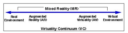
    [20] P. Milgram and A. F. Kishino, Taxonomy of mixed reality visual displays, IEICE T. Inform. Syst., (1994), 1321–1329.
    [21] K. C. Li, C. W. Tsai, C. T. Chen, et al., The design of immersive English learning environment using augmented reality, Process of 8th IEEE International Conference on UMEDIA, (2015), 174–179.
    [22] C. S. C. Dalim, A. Dey and T. Piumsomboon, TeachAR: An interactive augmented reality tool for teaching basic English to non-native children, Process of IEEE International Symposium on Mixed and Augmented Reality Adjunct, (2016), 67–72.
    [23] F. Sorrentino, L. D. Spano and R. Scateni, Speaky notes learn languages with augmented reality, Process of IEEE International Conference Interactive Mobile Communication Technologies and Learning (IMCL), (2015), 56–61.
  • This article has been cited by:

    1. Noreen Saba, Sana Maqsood, Muhammad Asghar, Ghulam Mustafa, Faheem Khan, An extended Mittag Leffler function in terms of extended Wright complex hypergeometric function, 2025, 117, 11100168, 364, 10.1016/j.aej.2024.12.065
  • Reader Comments
  • © 2019 the Author(s), licensee AIMS Press. This is an open access article distributed under the terms of the Creative Commons Attribution License (http://creativecommons.org/licenses/by/4.0)
通讯作者: 陈斌, bchen63@163.com
  • 1. 

    沈阳化工大学材料科学与工程学院 沈阳 110142

  1. 本站搜索
  2. 百度学术搜索
  3. 万方数据库搜索
  4. CNKI搜索

Metrics

Article views(5557) PDF downloads(658) Cited by(10)

Figures and Tables

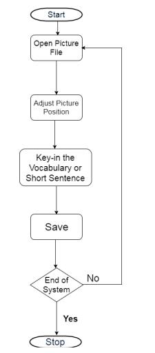
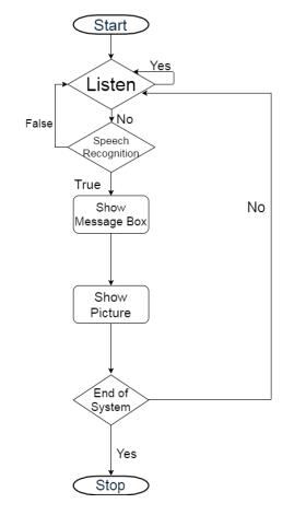
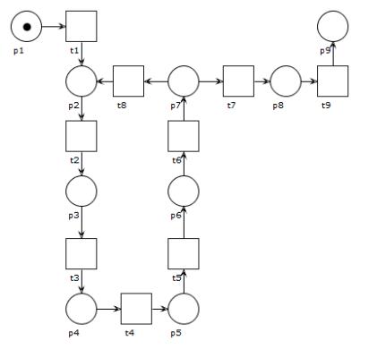
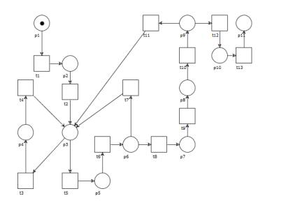
Figures(33)  /  Tables(7)

/

DownLoad:  Full-Size Img  PowerPoint
Return
Return

Catalog