The objective of the present paper is to solve a one-dimensional quasilinear parabolic singularly perturbed problem with a discontinuous source term. Due to the presence of such a discontinuity, an interior layer exists at the location of the discontinuity. The problem is solved by discretizing the spatial variable on a piecewise uniform Shishkin mesh using the standard upwind approach, while the backward Euler scheme is employed on a uniform mesh to discretize the time variable. The method is $ \varepsilon $-uniformly convergent, providing first-order convergence in the time domain and almost first-order convergence in the spatial variable. To validate the theoretical findings, the scheme was tested by numerically solving two examples.
Citation: Ruby, Vembu Shanthi, Higinio Ramos. A numerical approach to approximate the solution of a quasilinear singularly perturbed parabolic convection diffusion problem having a non-smooth source term[J]. AIMS Mathematics, 2025, 10(3): 6827-6852. doi: 10.3934/math.2025313
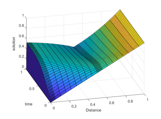
The objective of the present paper is to solve a one-dimensional quasilinear parabolic singularly perturbed problem with a discontinuous source term. Due to the presence of such a discontinuity, an interior layer exists at the location of the discontinuity. The problem is solved by discretizing the spatial variable on a piecewise uniform Shishkin mesh using the standard upwind approach, while the backward Euler scheme is employed on a uniform mesh to discretize the time variable. The method is $ \varepsilon $-uniformly convergent, providing first-order convergence in the time domain and almost first-order convergence in the spatial variable. To validate the theoretical findings, the scheme was tested by numerically solving two examples.

| [1] | P. A. Markowich, C. A. Ringhofer, C. Schmeiser, Semiconductor equations, Springer Vienna, 2012. |
| [2] | E. P. Doolan, J. J. H. Miller, W. H. A. Schilders, Uniform numerical methods for problems with initial and boundary layers, Boole Press, 1980. |
| [3] | P. A. Farrell, A. Hegarty, J. J. H. Miller, E. O'Riordan, G. I. Shishkin, Robust computational techniques for boundary layers, Chapman and hall/CRC, 2000. https://doi.org/10.1201/9781482285727 |
| [4] | J. J. H. Miller, E. O'Riordan, G. I. Shishkin, Fitted numerical methods for singular perturbation problems: error estimates in the maximum norm for linear problems in one and two dimensions, World scientific, 2012. https://doi.org/10.1142/8410 |
| [5] | H. G. Roos, M. Stynes, L. Tobiska, Robust numerical methods for singularly perturbed differential equations, Springer Series in Computational Mathematics, Vol. 24, 2 Eds., Springer, Berlin, 2008. https://doi.org/10.1007/978-3-540-34467-4 |
| [6] |
P. A. Farrell, A. F. Hegarty, J. J. H. Miller, E. O'Riordan, G. I. Shishkin, Global maximum norm parameter-uniform numerical method for a singularly perturbed convection-diffusion problem with discontinuous convection coefficient, Math. Comput. Model., 40 (2004), 1375–1392. https://doi.org/10.1016/j.mcm.2005.01.025 doi: 10.1016/j.mcm.2005.01.025

|
| [7] |
P. A. Farrell, E. O'Riordan, G. I. Shishkin, A class of singularly perturbed quasilinear differential equations with interior layers, Math. Comp., 78 (2009), 103–127. https://doi.org/10.1090/S0025-5718-08-02157-1 doi: 10.1090/S0025-5718-08-02157-1
|
| [8] |
S. C. S. Rao, A. K. Chaturvedi, Analysis and implementation of a computational technique for a coupled system of two singularly perturbed parabolic semilinear reaction–diffusion equations having discontinuous source terms, Commun. Nonlinear Sci. Numer. Simul., 108 (2022), 106232. https://doi.org/10.1016/j.cnsns.2021.106232 doi: 10.1016/j.cnsns.2021.106232
|
| [9] |
Ruby, V. Shanthi, H. Ramos, Numerical analysis for a weakly coupled system of singularly perturbed quasilinear problem with non-smooth data, J. Comput. Sci., 85 (2025), 102475. https://doi.org/10.1016/j.jocs.2024.102475 doi: 10.1016/j.jocs.2024.102475
|
| [10] | H. Schlichting, K. Gersten, Boundary-layer theory, 9 Eds., Springer Berlin, Heidelberg, 2017. https://doi.org/10.1007/978-3-662-52919-5 |
| [11] | C. M. Bender, S. A. Orszag, Advanced mathematical methods for scientists and engineers Ⅰ: asymptotic methods and perturbation theory, Springer Science & Business Media, 2013. |
| [12] | P. Kokotović, H. K. Khalil, J. O'Reilly, Singular perturbation methods in control: analysis and design, SIAM, 1999. |
| [13] | P. A. Markowich, The stationary semiconductor device equations, Springer Vienna, 1986. https://doi.org/10.1007/978-3-7091-3678-2 |
| [14] | S. Selberherr, Analysis and simulation of semiconductor devices, Springer Science & Business Media, 2012. |
| [15] | O. A. Ladyženskaja, V. A. Solonnikov, N. N. Ural'ceva, Linear and quasi-linear equations of parabolic type, In: Translations of mathematical monographs, Vol. 23, American Mathematical Society, 1968. |
| [16] |
E. O'Riordan, G. I. Shishkin, Singularly perturbed parabolic problems with non-smooth data, J. Comput. Appl. Math., 166 (2004), 233–245. https://doi.org/10.1016/j.cam.2003.09.025 doi: 10.1016/j.cam.2003.09.025
|
| [17] |
K. Mukherjee, S. Natesan, $\varepsilon$-Uniform error estimate of hybrid numerical scheme for singularly perturbed parabolic problems with interior layers, Numer. Algor., 58 (2011), 103–141. https://doi.org/10.1007/s11075-011-9449-6 doi: 10.1007/s11075-011-9449-6
|
| [18] | S. R. Bernfeld, V. Lakshmikantham, An introduction to nonlinear boundary value problems, New York: Academic Press, 1974. |
| [19] | J. J. H. Miller, E. O'Riordan, G. I. Shishkin, L. P. Shishkina Fitted mesh methods for problems with parabolic boundary layers, Math. Proc. Royal Irish Acad., 98A (1998), 173–190. |
| [20] |
M. Stynes, E. O'Riordan, Uniformly convergent difference schemes for singularly perturbed parabolic diffusion-convection problems without turning points, Numer. Math., 55 (1989), 521–544. https://doi.org/10.1007/BF01398914 doi: 10.1007/BF01398914
|
| [21] |
P. A. Farrell, A. F. Hegarty, J. J. H. Miller, E. O'Riordan, G. I. Shishkin, Singularly perturbed convection–diffusion problems with boundary and weak interior layers, J. Comput. Appl. Math., 166 (2004), 133–151. https://doi.org/10.1016/j.cam.2003.09.033 doi: 10.1016/j.cam.2003.09.033
|
| [22] | H. G Roos, M. Stynes, L. Tobiska, Numerical methods for singularly perturbed differential equations: convection-diffusion and flow problems, Springer Berlin, Heidelberg, 1996. https://doi.org/10.1007/978-3-662-03206-0 |
| [23] |
E. O'Riordan, J. Quinn, A linearised singularly perturbed convection–diffusion problem with an interior layer, Appl. Numer. Math., 98 (2015), 1–17. https://doi.org/10.1016/j.apnum.2015.08.002 doi: 10.1016/j.apnum.2015.08.002
|
| [24] | J. W. Thomas, Numerical partial differential equations: finite difference methods, Springer Science & Business Media, 2013. |

Figures(2) / Tables(6)

Ruby, Vembu Shanthi, Higinio Ramos. A numerical approach to approximate the solution of a quasilinear singularly perturbed parabolic convection diffusion problem having a non-smooth source term[J]. AIMS Mathematics, 2025, 10(3): 6827-6852. doi: 10.3934/math.2025313


 DownLoad: