In this research, we are examining the stochastic modified Korteweg-de Vries (SMKdV) equation forced in the Itô sense by multiplicative noise. We use an appropriate transformation to convert the SMKdV equation to another MKdV equation with random variable coefficients (MKdV-RVCs). We use the generalizing Riccati equation mapping and Jacobi elliptic functions methods in order to acquire new trigonometric, hyperbolic, and rational solutions for MKdV-RVCs. After that, we can get the solutions to the SMKdV equation. To our knowledge, this is the first time we have assumed that the solution of the wave equation for the SMKdV equation is stochastic, since all earlier research assumed that it was deterministic. Furthermore, we provide different graphic representations to show the influence of multiplicative noise on the exact solutions of the SMKdV equation.
Citation: Wael W. Mohammed, Farah M. Al-Askar. New stochastic solitary solutions for the modified Korteweg-de Vries equation with stochastic term/random variable coefficients[J]. AIMS Mathematics, 2024, 9(8): 20467-20481. doi: 10.3934/math.2024995
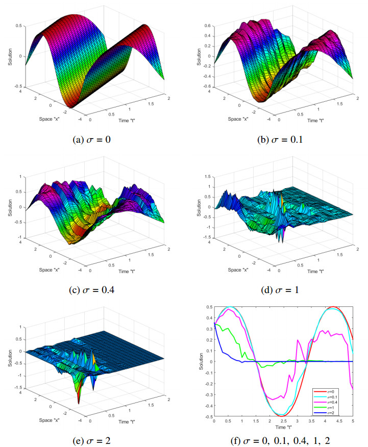
In this research, we are examining the stochastic modified Korteweg-de Vries (SMKdV) equation forced in the Itô sense by multiplicative noise. We use an appropriate transformation to convert the SMKdV equation to another MKdV equation with random variable coefficients (MKdV-RVCs). We use the generalizing Riccati equation mapping and Jacobi elliptic functions methods in order to acquire new trigonometric, hyperbolic, and rational solutions for MKdV-RVCs. After that, we can get the solutions to the SMKdV equation. To our knowledge, this is the first time we have assumed that the solution of the wave equation for the SMKdV equation is stochastic, since all earlier research assumed that it was deterministic. Furthermore, we provide different graphic representations to show the influence of multiplicative noise on the exact solutions of the SMKdV equation.

| [1] |
S. Tanaka, Modified Korteweg-de Vries equation and scattering theory, P. Jpn. Acad., 48 (1972), 466–469. http://dx.doi.org/10.3792/pja/1195519590 doi: 10.3792/pja/1195519590

|
| [2] |
A. H. Khater, O. H. El-Kalaawy, D. K. Callebaut, Bäcklund transformations and exact solutions for Alfvén solitons in a relativistic electron-positron plasma, Phys. Scripta, 58 (1998), 545. http://dx.doi.org/10.1088/0031-8949/58/6/001 doi: 10.1088/0031-8949/58/6/001
|
| [3] |
Z. P. Li, Y. C. Liu, Analysis of stability and density waves of traffic flow model in an ITS environment, Eur. Phys. J. B, 53 (2006), 367–374. https://doi.org/10.1140/epjb/e2006-00382-7 doi: 10.1140/epjb/e2006-00382-7
|
| [4] |
M. A. Helal, Soliton solution of some nonlinear partial differential equations and its applications in fluid mechanics, Chaos Solition. Fract., 13 (2002), 1917–1929. https://doi.org/10.1016/S0960-0779(01)00189-8 doi: 10.1016/S0960-0779(01)00189-8
|
| [5] | H. Leblond, D. Mihalache, Few-optical-cycle solitons: Modified Kortewegde Vries sine-Gordon equation versus other non-slowly-varying-envelopeapproximation models, Phys. Rev. A, 79 (2009). |
| [6] |
A. A. Elmandouha, A. G. Ibrahim, Bifurcation and travelling wave solutions for a (2+1)-dimensional KdV equation, J. Taibah Univ. Sci., 14 (2020), 139–147. https://doi.org/10.1080/16583655.2019.1709271 doi: 10.1080/16583655.2019.1709271
|
| [7] |
F. M. Al-Askar, C. Cesarano, W. W. Mohammed, Effects of the wiener process and beta derivative on the exact solutions of the kadomtsev-petviashvili equation, Axioms, 12 (2023), 748. https://doi.org/10.3390/axioms12080748 doi: 10.3390/axioms12080748
|
| [8] | N. Taghizadeh, Comparison of solutions of mKdV equation by using the first integral method and ($G^{\prime }/G$)-expansion method, Math. Aeterna, 2 (2012), 309–320. |
| [9] |
K. R. Raslan, The application of He's Exp-function method for mKdV and Burgers' equations with variable coefficients, Int. J. Nonlin. Sci., 7 (2009), 174–181. https://doi.org/10.1016/j.camwa.2009.03.019 doi: 10.1016/j.camwa.2009.03.019
|
| [10] | Y. Yang, Exact solutions of the mKdV equation, IOP Conference Series: Earth and Environmental Science, IOP Publishing, 769 (2021), 042040. https://doi.org/10.1088/1755-1315/769/4/042040 |
| [11] |
A. M. Wazwaz, The tanh method for generalized forms of nonlinear heat conduction and Burgers-Fisher equations, Appl. Math. Comput., 169 (2005), 321–338. https://doi.org/10.1016/j.amc.2004.09.054 doi: 10.1016/j.amc.2004.09.054
|
| [12] |
W. W. Mohammed, F. M. Al-Askar, C. Cesarano, The analytical solutions of the stochastic mKdV equation via the mapping method, Mathematics, 10 (2022), 4212. https://doi.org/10.3390/math10224212 doi: 10.3390/math10224212
|
| [13] |
C. Liu, Z. Li, The dynamical behavior analysis and the traveling wave solutions of the stochastic Sasa-Satsuma equation, Qual. Theory Dyn. Syst., 23 (2024), 157. https://doi.org/10.1007/s12346-024-01022-y doi: 10.1007/s12346-024-01022-y
|
| [14] |
Z. Li, C. Liu, Chaotic pattern and traveling wave solution of the perturbed stochastic nonlinear Schrödinger equation with generalized anti-cubic law nonlinearity and spatio-temporal dispersion, Results Phys., 56 (2024), 107305. https://doi.org/10.1016/j.rinp.2023.107305 doi: 10.1016/j.rinp.2023.107305
|
| [15] |
C. Liu, Z. Li, Multiplicative brownian motion stabilizes traveling wave solutions and dynamical behavior analysis of the stochastic Davey-Stewartson equations, Results Phys., 53 (2023), 106941. https://doi.org/10.1016/j.rinp.2023.106941 doi: 10.1016/j.rinp.2023.106941
|
| [16] |
S. Albosaily, E. M. Elsayed, M. D. Albalwi, M. Alesemi, W. W. Mohammed, The analytical stochastic solutions for the stochastic Potential Yu-Toda-Sasa-Fukuyama equation with conformable derivative using different methods, Fractal Fract., 7 (2023), 787. https://doi.org/10.3390/fractalfract7110787 doi: 10.3390/fractalfract7110787
|
| [17] |
M. Z. Baber, N. Ahmed, M. S. Iqbal, Exact solitary wave propagations for the stochastic Burgers' equation under the influence of white noise and its comparison with computational scheme, Sci. Rep., 14 (2024), 10629. https://doi.org/10.1038/s41598-024-58553-2 doi: 10.1038/s41598-024-58553-2
|
| [18] |
F. M. Al-Askar, C. Cesarano, W. W. Mohammed, The solitary solutions for the stochastic Jimbo-Miwa equation perturbed by White noise, Symmetry, 15 (2023), 1153. https://doi.org/10.3390/sym15061153 doi: 10.3390/sym15061153
|
| [19] |
W. W. Mohammed, F. M. Al-Askar, C. Cesarano, On the dynamical behavior of solitary waves for coupled stochastic Korteweg-De Vries equations, Mathematics, 11 (2023), 3506. https://doi.org/10.3390/math11163506 doi: 10.3390/math11163506
|
| [20] |
A. Elmandouh, E. Fadhal, Bifurcation of exact solutions for the space-fractional stochastic modified Benjamin-Bona-Mahony equation, Fractal Fract., 6 (2022), 718. https://doi.org/10.3390/fractalfract6120718 doi: 10.3390/fractalfract6120718
|
| [21] |
W. W. Mohammed, C. Cesarano, A. A. Elmandouh, I. Alqsair, R. Sidaoui, H. W. Alshammari, Abundant optical soliton solutions for the stochastic fractional fokas system using bifurcation analysis, Phys. Scripta, 99 (2024), 045233. https://doi.org/10.1088/1402-4896/ad30fd doi: 10.1088/1402-4896/ad30fd
|
| [22] | S. D. Zhu, The generalizing Riccati equation mapping method in non-linear evolution equation: Application to (2+1)-dimensional Boiti-Leon-Pempinelle equation, Chaos Solition. Fract., 37 (2008), 1335–1342. |
| [23] |
E. Fan, J. Zhang, Applications of the Jacobi elliptic function method to special-type nonlinear equations, Phys. Lett. A, 305 (2002), 383–392. https://doi.org/10.1016/S0375-9601(02)01516-5 doi: 10.1016/S0375-9601(02)01516-5
|


Figures(3)

Wael W. Mohammed, Farah M. Al-Askar. New stochastic solitary solutions for the modified Korteweg-de Vries equation with stochastic term/random variable coefficients[J]. AIMS Mathematics, 2024, 9(8): 20467-20481. doi: 10.3934/math.2024995


 DownLoad: