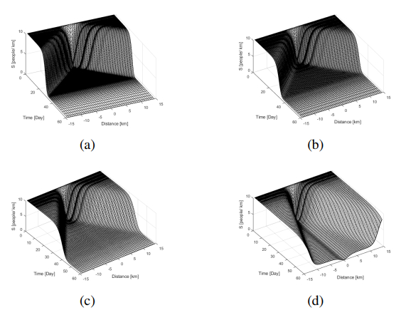
Coronavirus spread in Wuhan, China, in December 2019. A few weeks later, the virus was present in over 100 countries around the globe. Governments have adopted extreme measures to contain the spreading virus. Quarantine is considered the most effective way to control the spreading speed of COVID-19. In this study, a mathematical model is developed to explore the influence of quarantine and the latent period on the spatial spread of COVID-19. We use the mathematical model with quarantine, and delay to predict the spreading speed of the virus. In particular, we transform the model to a single integral equation and then apply the Laplace transform to find implicit equations for the spreading speeds. The basic reproduction number of COVID-19 is also found and calculated. Numerical simulations are performed to confirm our theoretical results. To validate the proposed model, we compare our outcomes with the actual reported data published by the National Health Commission of China and the Health Commission of local governments. The model demonstrates good qualitative agreement with the actual data reported. The results show that delay and quarantine highly influence the spreading speeds of COVID-19. Also, we can only contain the disease if we quarantine $ 75 \% $ of the infected people.
Citation: Khalaf M. Alanazi. The asymptotic spreading speeds of COVID-19 with the effect of delay and quarantine[J]. AIMS Mathematics, 2024, 9(7): 19397-19413. doi: 10.3934/math.2024945
Coronavirus spread in Wuhan, China, in December 2019. A few weeks later, the virus was present in over 100 countries around the globe. Governments have adopted extreme measures to contain the spreading virus. Quarantine is considered the most effective way to control the spreading speed of COVID-19. In this study, a mathematical model is developed to explore the influence of quarantine and the latent period on the spatial spread of COVID-19. We use the mathematical model with quarantine, and delay to predict the spreading speed of the virus. In particular, we transform the model to a single integral equation and then apply the Laplace transform to find implicit equations for the spreading speeds. The basic reproduction number of COVID-19 is also found and calculated. Numerical simulations are performed to confirm our theoretical results. To validate the proposed model, we compare our outcomes with the actual reported data published by the National Health Commission of China and the Health Commission of local governments. The model demonstrates good qualitative agreement with the actual data reported. The results show that delay and quarantine highly influence the spreading speeds of COVID-19. Also, we can only contain the disease if we quarantine $ 75 \% $ of the infected people.

| [1] |
K. M. Alanazi, Modeling and simulating an epidemic in two dimensions with an application regarding COVID-19, Computation, 12 (2024), 34. https://doi.org/10.3390/computation12020034 doi: 10.3390/computation12020034

|
| [2] |
K. M. Alanazi, Z. Jackiewicz, H. R. Thieme, Numerical simulations of spread of rabies in a spatially distributed fox population, Math. Comput. Simul., 159 (2019), 161–182. https://doi.org/10.1016/j.matcom.2018.11.010 doi: 10.1016/j.matcom.2018.11.010
|
| [3] |
K. M. Alanazi, Z. Jackiewicz, H. R. Thieme, Numerical simulations of the spread of rabies in two-dimensional space, Appl. Numer. Math., 135 (2019), 87–98. https://doi.org/10.1016/j.apnum.2018.08.009 doi: 10.1016/j.apnum.2018.08.009
|
| [4] |
K. M. Alanazi, Z. Jackiewicz, H. R. Thieme, Spreading speeds of rabies with territorial and diffusing rabid foxes, Discr. Cont. Dyn. Syst. Ser. B, 25 (2020), 2143. https://doi.org/10.3934/dcdsb.2019222 doi: 10.3934/dcdsb.2019222
|
| [5] |
C. Anastassopoulou, L. Russo, L. Tsakris, C. Siettos, Modelling and forecasting of the COVID-19 outbreak, PLoS One, 15 (2020), e0230405. https://doi.org/10.1371/journal.pone.0230405 doi: 10.1371/journal.pone.0230405
|
| [6] | J. Arino, S. Portet, A simple model for COVID-19, Infect. Dis. Model., 5 (2020), 309–315. |
| [7] | D. G. Aronson, The asymptotic speed of propagation of a simple epidemic, Nonlinear Diffus., 14, (1977), 1–23. |
| [8] | D. G. Aronson, H. F. Weinberger, Nonlinear diffusion in population genetics, combustion, and nerve pulse propagation, Partial Differ. Equ. Related Topics, 446, (1975), 5–49. |
| [9] |
D. G. Aronson, H. F. Weinberger, Multidimensional nonlinear diffusion arising in population genetics, Adv. Math., 30 (1978), 33–76. https://doi.org/10.1016/0001-8708(78)90130-5 doi: 10.1016/0001-8708(78)90130-5
|
| [10] |
A. Babaei, M. Ahmadi, H. Jafari, A. Liya, A mathematical model to examine the effect of quarantine on the spread of coronavirus, Chaos Solitons Fract., 142 (2021), 110418. https://doi.org/10.1016/j.chaos.2020.110418 doi: 10.1016/j.chaos.2020.110418
|
| [11] |
B. Batista, Minimizing disease spread on a quarantined cruise ship: a model of COVID-19 with asymptomatic infections, Math. Biosci., 329 (2020), 108442. https://doi.org/10.1016/j.mbs.2020.108442 doi: 10.1016/j.mbs.2020.108442
|
| [12] |
H. Berestycki, J. M. Roquejoffre, L. Rossi, Propagation of epidemics along lines with fast diffusion, Bull. Math. Biol., 83 (2021), 2. https://doi.org/10.1007/s11538-020-00826-8 doi: 10.1007/s11538-020-00826-8
|
| [13] |
J. Chen, Pathogenicity and transmissibility of 2019-nCoV-a quick overview and comparison with other emerging viruses, Microbes Infect., 22 (2020), 69–71. https://doi.org/10.1016/j.micinf.2020.01.004 doi: 10.1016/j.micinf.2020.01.004
|
| [14] |
Q. Cui, Z. Hu, Y. Li, J. Han, Z. Teng, J. Qian, Dynamic variations of the COVID-19 disease at different quarantine strategies in Wuhan and mainland China, J. Infect. Publ. Heal., 13 (2020), 849–855. https://doi.org/10.1016/j.jiph.2020.05.014 doi: 10.1016/j.jiph.2020.05.014
|
| [15] | O. Diekmann, Limiting behaviour in an epidemic model, Nonlinear Anal., 1 (1977), 459–470. |
| [16] |
O. Diekmann, Thresholds and travelling waves for the geographical spread of infection, J. Math. Biol., 6 (1978), 109–130. https://doi.org/10.1007/BF02450783 doi: 10.1007/BF02450783
|
| [17] |
O. Diekmann, Run for your life. A note on the asymptotic speed of propagation of an epidemic, J. Diff. Equ., 33 (1979), 5873. https://doi.org/10.1016/0022-0396(79)90080-9 doi: 10.1016/0022-0396(79)90080-9
|
| [18] |
R. Engbert, M. M. Rabe, R. Kliegl, S. Reich, Sequential data assimilation of the stochastic SEIR epidemic model for regional COVID-19 dynamics, Bull. Math. Biol., 83 (2021), 1. https://doi.org/10.1007/s11538-020-00834-8 doi: 10.1007/s11538-020-00834-8
|
| [19] |
Y. Feng, Q. Li, X. Tong, R. Wang, S. Zhai, C. Gao, et al., Spatiotemporal spread pattern of the COVID-19 cases in China, PLoS One, 15 (2020), e0244351. https://doi.org/10.1371/journal.pone.0244351 doi: 10.1371/journal.pone.0244351
|
| [20] |
M. Gatto, E. Bertuzzo, L. Mari, S. Miccoli, L. Carraro, R. Casagrandi, et al., Spread and dynamics of the COVID-19 epidemic in Italy: effects of emergency containment measures, Proc. Natl. Academy Sci., 117 (2020), 10484–10491. https://doi.org/10.1073/pnas.2004978117 doi: 10.1073/pnas.2004978117
|
| [21] |
Y. Guo, T. Li, Modeling the competitive transmission of the Omicron strain and Delta strain of COVID-19, J. Math. Anal. Appl., 526 (2023), 127283. https://doi.org/10.1016/j.jmaa.2023.127283 doi: 10.1016/j.jmaa.2023.127283
|
| [22] |
J. Hellewell, S. Abbott, A. Gimma, N. I. Bosse, C. I Jarvis, T. W. Russell, et al., Feasibility of controlling COVID-19 outbreaks by isolation of cases and contacts, Lancet Global Heal., 8 (2020), e488–e496. https://doi.org/10.1016/S2214-109X(20)30074-7 doi: 10.1016/S2214-109X(20)30074-7
|
| [23] |
C. Hou, J. Chen, Y. Zhou, L. Hua, J. Yuan, S. He, et al., The effectiveness of quarantine of Wuhan city against the Corona Virus Disease 2019 (COVID‐19): a well‐mixed SEIR model analysis, J. Medical Virol., 92 (2020), 841–848. https://doi.org/10.1002/jmv.25827 doi: 10.1002/jmv.25827
|
| [24] |
K. K. Hwang, C. J. Edholm, O. Saucedo, L. J. S. Allen, N. Shakiba, A hybrid epidemic model to explore stochasticity in COVID-19 dynamics, Bull. Math. Biol., 84 (2022), 91. https://doi.org/10.1007/s11538-022-01030-6 doi: 10.1007/s11538-022-01030-6
|
| [25] |
E. Iboi, O. O. Sharomi, C. Ngonghala, A. B. Gumel, Mathematical modeling and analysis of COVID-19 pandemic in Nigeria, Math. Biosci. Eng., 17 (2020), 7192–7220. https://doi.org/10.3934/mbe.2020369 doi: 10.3934/mbe.2020369
|
| [26] |
A. Kouidere, L. E. Youssoufi, H. Ferjouchia, O. Balatif, M. Rachik, Optimal control of mathematical modeling of the spread of the COVID-19 pandemic with highlighting the negative impact of quarantine on diabetics people with cost-effectiveness, Chaos Solitons Fract., 145 (2021), 110777. https://doi.org/10.1016/j.chaos.2021.110777 doi: 10.1016/j.chaos.2021.110777
|
| [27] |
A. J. Kucharski, T. W. Russell, C. Diamond, Y. Liu, J. Edmunds, S. Funk, et al., Early dynamics of transmission and control of COVID-19: a mathematical modelling study, Lancet Infect. Dis., 20 (2020), 553–558. https://doi.org/10.1016/S1473-3099(20)30144-4 doi: 10.1016/S1473-3099(20)30144-4
|
| [28] |
Q. Li, X. Guan, P. Wu, X. Wang, L. Zhou, Y. Tong, et al., Early transmission dynamics in Wuhan, China, of novel coronavirus–infected pneumonia, New England J. Medic., 382 (2020), 1199–1207. https://doi.org/10.1056/NEJMoa2001316 doi: 10.1056/NEJMoa2001316
|
| [29] |
T. Li, Y. Guo, Modeling and optimal control of mutated COVID-19 (Delta strain) with imperfect vaccination, Chaos Solitons Fract., 156 (2022), 111825. https://doi.org/10.1016/j.chaos.2022.111825 doi: 10.1016/j.chaos.2022.111825
|
| [30] |
Q. Lin, S. Zhao, D. Gao, Y. Lou, S. Yang, S. S. Musa, et al., A conceptual model for the coronavirus disease 2019 (COVID-19) outbreak in Wuhan, China with individual reaction and governmental action, Int. J. Infect. Dis., 93 (2020), 211–216. https://doi.org/10.1016/j.ijid.2020.02.058 doi: 10.1016/j.ijid.2020.02.058
|
| [31] |
J. M. Read, J. R. Bridgen, D. A. Cummings, A. Ho, C. P. Jewell, Novel coronavirus 2019-nCoV (COVID-19): early estimation of epidemiological parameters and epidemic size estimates, Philos. T. Royal Soc. B, 376 (2021), 20200265. https://doi.org/10.1098/rstb.2020.0265 doi: 10.1098/rstb.2020.0265
|
| [32] | A. Remuzzi, G. Remuzzi, COVID-19 and Italy: what next? Lancet, 395 (2020), 1225–1228. https://doi.org/10.1016/S0140-6736(20)30627-9 |
| [33] | S. Ruan, Spatial-Temporal Dynamics in Nonlocal Epidemiological Models, Berlin: Springer, 2007. |
| [34] |
M. A. Safi, A. B. Gumel, Dynamics of a model with quarantine-adjusted incidence and quarantine of susceptible individuals, J. Math. Anal. Appl., 399 (2013), 565–575. https://doi.org/10.1016/j.jmaa.2012.10.015 doi: 10.1016/j.jmaa.2012.10.015
|
| [35] |
B. Tang, F. Xia, S. Tang, N. L. Bragazzi, Q. Li, X. Sun, et al., The effectiveness of quarantine and isolation determine the trend of the COVID-19 epidemic in the final phase of the current outbreak in China, Int. J. Infect. Dis., 96 (2020), 288–293. https://doi.org/10.1016/j.ijid.2020.05.113 doi: 10.1016/j.ijid.2020.05.113
|
| [36] | J. Tanimoto, Sociophysics Approach to Epidemics, Singapore: Springer, 2021. |
| [37] |
H. R. Thieme, A model for the spatial spread of an epidemic, J. Math. Biol., 4 (1977), 337–351. https://doi.org/10.1007/BF00275082 doi: 10.1007/BF00275082
|
| [38] |
H. R. Thieme, Asymptotic estimates of the solutions of nonlinear integral equations and asymptotic speeds for the spread of populations, J. Reine Angew. Math., 306 (1979), 94–121. https://doi.org/10.1515/crll.1979.306.94 doi: 10.1515/crll.1979.306.94
|
| [39] | H. R. Thieme, Mathematics in Population Biology, Princeton: Princeton University Press, 2003. |
| [40] |
H. R. Thieme, X. Q. Zhao, Asymptotic speeds of spread and traveling waves for integral equations and delayed reaction-diffusion models, J. Diff. Equ., 195 (2003), 430–470. https://doi.org/10.1016/S0022-0396(03)00175-X doi: 10.1016/S0022-0396(03)00175-X
|
| [41] |
A. Viguerie, G. Lorenzo, F. Auricchio, D. Baroli, T. J. Hughes, A. Patton, et al., Simulating the spread of COVID-19 via a spatially-resolved susceptible-exposed-infected-recovered-deceased (SEIRD) model with heterogeneous diffusion, Appl. Math. Lett., 111 (2021), 106617. https://doi.org/10.1016/j.aml.2020.106617 doi: 10.1016/j.aml.2020.106617
|
| [42] |
Y. Wang, Y. Wang, Y. Chen, Q. Qin, Unique epidemiological and clinical features of the emerging 2019 novel coronavirus pneumonia (COVID‐19) implicate special control measures, J. Medical Virol., 92 (2020), 568–576. https://doi.org/10.1002/jmv.25748 doi: 10.1002/jmv.25748
|
| [43] |
F. Wei, R. Zhou, Z. Jin, S. Huang, Z. Peng, J. Wang, et al., COVID-19 transmission driven by age-group mathematical model in Shijiazhuang City of China, Infect. Dis. Model., 8 (2023), 1050–1062. https://doi.org/10.1016/j.idm.2023.08.004 doi: 10.1016/j.idm.2023.08.004
|
| [44] |
J. T. Wu, K. Leung, G. M. Leung, Nowcasting and forecasting the potential domestic and international spread of the 2019-nCoV outbreak originating in Wuhan, China: a modelling study, Lancet, 395 (2020), 689–697. https://doi.org/10.1016/S0140-6736(20)30260-9 doi: 10.1016/S0140-6736(20)30260-9
|
| [45] |
R. Xu, H. Rahmandad, M. Gupta, C. DiGennaro, N. Ghaffarzadegan, H. Amini, et al., Weather, air pollution, and SARS-CoV-2 transmission: a global analysis, Lancet Planetary Heal., 5 (2021), e671–e680. https://doi.org/10.1016/S2542-5196(21)00202-3 doi: 10.1016/S2542-5196(21)00202-3
|
| [46] |
S. Zhao, Q. Lin, J. Ran, S. S. Musa, G. Yang, W. Wang, et al., Preliminary estimation of the basic reproduction number of novel coronavirus (2019-nCoV) in China, from 2019 to 2020: a data-driven analysis in the early phase of the outbreak, Int. J. Infect. Dis., 92 (2020), 214–217. https://doi.org/10.1016/j.ijid.2020.01.050 doi: 10.1016/j.ijid.2020.01.050
|
| [47] |
C. C. Zhu, J. Zhu, Dynamic analysis of a delayed COVID-19 epidemic with home quarantine in temporal-spatial heterogeneous via global exponential attractor method, Chaos Solitons Fract., 143 (2021), 110546. https://doi.org/10.1016/j.chaos.2020.110546 doi: 10.1016/j.chaos.2020.110546
|


Figures(4) / Tables(8)

Khalaf M. Alanazi. The asymptotic spreading speeds of COVID-19 with the effect of delay and quarantine[J]. AIMS Mathematics, 2024, 9(7): 19397-19413. doi: 10.3934/math.2024945


 DownLoad: